How to Train Your Dragon (Detector)

A general guide to building high-quality deep learning datasets and models using ClearML and FiftyOne

Often thought to be the stuff of legends, we aim to shed light on a mythical entity. Dragons? No… An effective and repeatable data-centric machine learning workflow, of course! It seems that many machine learning researchers and engineers these days are focused on developing the optimal model architecture for their tasks.

In reality, the most surefire way to develop a high-performing model is to meticulously understand, track, and improve your datasets and experimental results.

In this post, we will walk through the process of developing a computer vision model and dataset in a repeatable and effective way utilizing ClearML and FiftyOne. Specifically, we will be training the object detection model DETR on a dataset of dragon images, though the general workflow presented is extensible to nearly any computer vision and machine learning task.

FiftyOne is an open-source tool for building high-quality datasets and computer vision models with a powerful API and intuitive App letting you quickly understand the quality of your dataset, find your model’s failure modes, and improve your datasets and models. On the other hand, ClearML is an open-source platform that automates and simplifies developing and managing machine learning solutions through an end-to-end MLOps suite allowing you to focus on developing your ML code and automation, while ClearML ensures your work is reproducible and scalable.

ClearML and FiftyOne go hand-in-hand with one another in your machine learning workflows. The combination of flexible, hands-on visualization and analysis of data and model results of FiftyOne combined with the experimental result tracking of ClearML produces a system that lets you quickly explore and improve your datasets while also persisting all of the changes and progress made to achieving a high-performing model.

Follow Along in Colab

You can follow along with this entire post directly in your browser through this Google Colab notebook!

The Tale of the Data and the Model FAIR

To keep things interesting, we created a whole new dataset especially for the occasion: dragons! We gathered 115 images of dragons and annotated them. Interestingly they are both cartoon-style dragons and more ‘realistic’ dragons.

To start things out, let’s download the dataset from here. For the detector, we used Meta (Facebook) research’s DETR, an object detection network based on the popular transformers architecture.

Integrating ClearML Experiment Tracking

ClearML experiment tracking works out of the box with most model training frameworks, including facebook’s own detectron2. Most things or imports are still tracked automagically using only the 2 magic lines (which we will cover below), but we also wanted to show how you can track specific metrics or images manually if required.

DETRs original codebase keeps track of training metrics in a .txt file and does not integrate with any additional tools like tensorboard. So let’s change that by adding only a few lines to make ClearML track our training runs automatically. This way, we can keep making the model better in an efficient way.

To get started with ClearML, go to the community server and get a ClearML account, or set up your own ClearML server as described here. This server will keep track of and consolidate all your code, models, data, and output.

After you have the server set up, it’s just a few commands before we can get cracking!

First of all, get the ClearML python package.

pip install clearml

Now we need to let your computer know where your server is.

clearml-init

This command will set up the connection from your local PC to the ClearML server. It will ask you for your ClearML configuration. You can get this info from the Profile page in your ClearML server.

2 magical lines

With only 2 lines of python code, we can already start tracking a lot! We add the following 2 lines of code to the top of the main.py file in the DETR repository. Every time we call this training script, ClearML will create a new task and log as much as it can.

# Initialise a clearML task and its corresponding logger
from clearml import Task
task = Task.init(project_name='dragon_detector', task_name=f'DETR')

These 2 lines will already track a lot of information, they will track:

• Artifacts (like saved models and checkpoints)
• Source code and packages information
• Configuration and hyperparameters
• Other info (runtime, hardware specs, etc.)
• Console output

Adding Manual Information

When using a framework like detectron2, these 2 lines are all you need. But this time, we’re training DETR using raw PyTorch and no additional tools like tensorboard, so we have to do a little more work ourselves.

For our own information to the experiment, we need a logger, which can be made as such:

logger = task.get_logger()

And now, we’re ready to add whatever information we desire to the experiment!

Adding scalars to the mix

Scalars are any type of value that we want to track and plot later down the line. In most cases, these will be training output values such as losses and accuracy metrics.

The original DETR implementation already logs the scalars we want to a .txt file, so all we have to do, is capture these parameters and add them to the ClearML task using the logger.report_scalar function.

# This code was already in DETR and keeps track of training metrics
test_stats, coco_evaluator = evaluate(
    model, criterion, postprocessors, data_loader_val, base_ds, device, args.output_dir
)
log_stats = {**{f'train_{k}': v for k, v in train_stats.items()},
             **{f'test_{k}': v for k, v in test_stats.items()},
             'epoch': epoch,
             'n_parameters': n_parameters}

# We add these lines to capture those training metrics in clearML
# Add all metrics except for coco_eval_bbox,
# since that is a bbox and not a scalar.
for key, value in log_stats.items():
    if 'coco_eval_bbox' in key:
        continue
    logger.report_scalar(title=key, series=key, value=value, iteration=epoch)

# This is where DETR normally writes these values to a txt file
if args.output_dir and utils.is_main_process():
    with (output_dir / "log.txt").open("a") as f:
        f.write(json.dumps(log_stats) + "\n")

Debug samples as the proverbial cherry on top

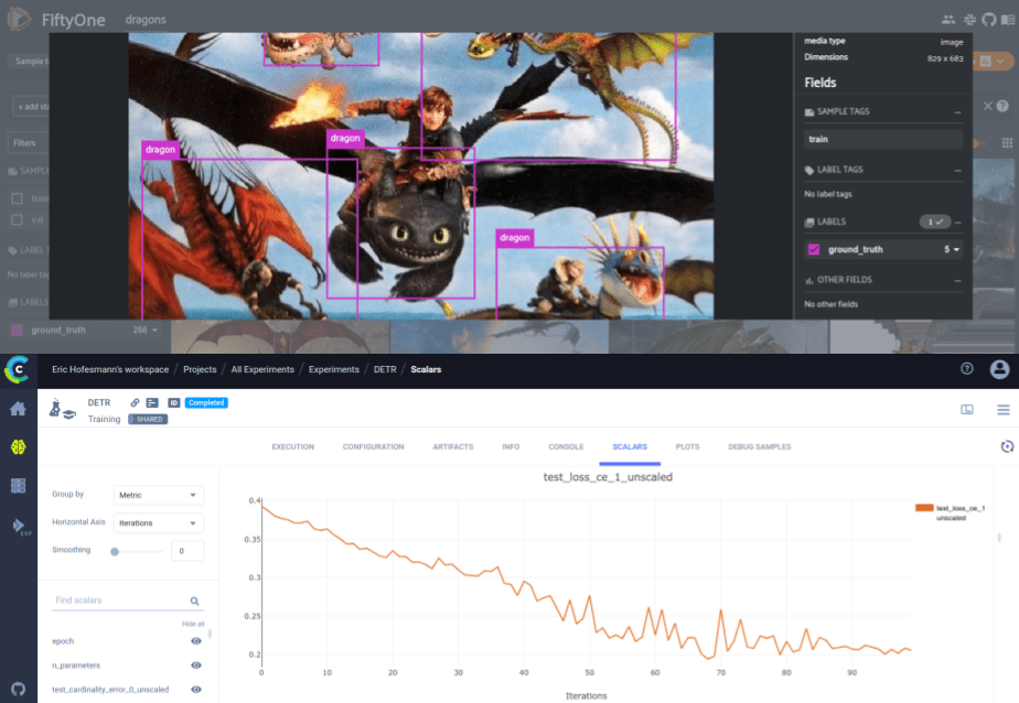
Debug samples are images that can be logged in much the same way as scalars. ClearML will pick up a matplotlib imshow image using the logger.report_matplotlib_figure function. In this case, we added a function that runs the model on the validation set at the end of training and log the annotated images to the experiment, to provide a quick glance at how well the model performs.

def plot_image_results(pil_img, prob, boxes, classes, logger, img_name):
    # colors for visualization
    colors = [[0.000, 0.447, 0.741], [0.850, 0.325, 0.098], [0.929, 0.694, 0.125],
              [0.494, 0.184, 0.556], [0.466, 0.674, 0.188], [0.301, 0.745, 0.933]]
    colors = colors * 100
    figure = plt.figure(figsize=(16,10))
    plt.imshow(pil_img)
    ax = plt.gca()
    for p, (xmin, ymin, xmax, ymax), c in zip(prob, boxes.tolist(), colors):
        ax.add_patch(plt.Rectangle((xmin, ymin), xmax - xmin, ymax - ymin,
                                   fill=False, color=c, linewidth=3))
        cl = p.argmax()
        text = f'{classes[cl]}: {p[cl]:0.2f}'
        ax.text(xmin, ymin, text, fontsize=15,
                bbox=dict(facecolor='yellow', alpha=0.5))
    plt.axis('off')
    logger.report_matplotlib_figure('Evaluation Results', img_name, figure,
                                    iteration=None, report_image=True,
                                    report_interactive=False)

Now we can easily train DETR in whatever way we want and be sure we captured all the relevant metrics. We can also always recreate our best experiments thanks to our comprehensive logging.

If we want to dig deeper and debug our model’s performance meticulously, we can analyze it using FiftyOne!

Digging in with FiftyOne

To start, let’s install FiftyOne:

pip install fiftyone

The first step is to load the dataset into FiftyOne so we can take a look at it in the FiftyOne App. Loading any custom dataset into FiftyOne is as simple as writing a Python loop. However, since this dataset is already in COCO format, we can load the splits with just one line of code.

import fiftyone as fo

dataset_name = "dragons"
dataset_dir = "/path/to/dataset"

# Load the training dataset into FiftyOne and tag all samples with "train"
dataset = fo.Dataset.from_dir(
    dataset_type=fo.types.COCODetectionDataset,
    data_path= os.path.join(dataset_dir, "train"),
    labels_path= os.path.join(dataset_dir, "annotations/train.json"),
    name=dataset_name,
    tags="train",
)

# Add the validation data and tag the samples with "val"
dataset.add_dir(
    dataset_type=fo.types.COCODetectionDataset,
    data_path= os.path.join(dataset_dir, "val"),
    labels_path= os.path.join(dataset_dir, "annotations/val.json"),
    tags="val",
)

The launch_app() method launches the App directly in the output of this cell and also returns a Session instance, which you can subsequently use to interact programmatically with the App.

session = fo.launch_app(dataset)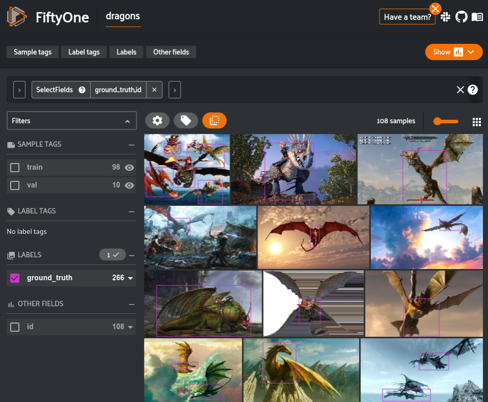

Loading predictions into FiftyOne

Similar to how you load ground truth labels into a FiftyOne Dataset, loading model predictions is as easy as writing a Python loop.

import fiftyone as fo

dataset = fo.load_dataset("dragons")
img_paths = ["/path/to/img1.png", ...]

# Ex. custom prediction format: [bbox, label, confidence]
predictions = [[[0.1,0.2,0.3,0.5], "car", 0.921], ...]

for img_path, img_preds in zip(img_paths, predictions):
    sample = dataset[img_path]
    dets = []
    for bbox, label, conf in img_preds:
        dets.append(
            fo.Detection(
                bounding_box=bbox,
                label=label,
                confidence=confidence,
            )
        )
    sample["predictions"] = fo.Detections(detections=dets)
    sample.save()
    
# View predictions in the App
session = fo.launch_app(dataset)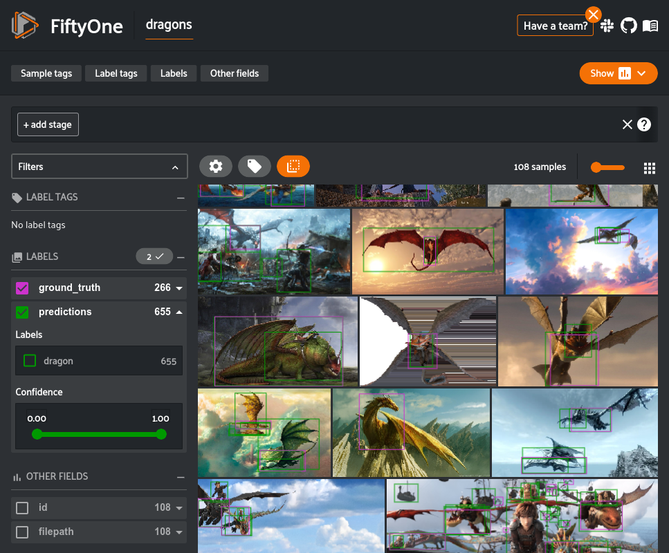

Once the predictions are in FiftyOne, we can easily export them in COCO format into a JSON file on disk.

# Export predictions from FiftyOne dataset to disk in COCO-formatted JSON
dataset.export(
    label_field="predictions",
    label_path="/path/to/coco_predictions.json",
    dataset_type=fo.types.COCODetectionDataset,
)

Evaluating and Filtering Results

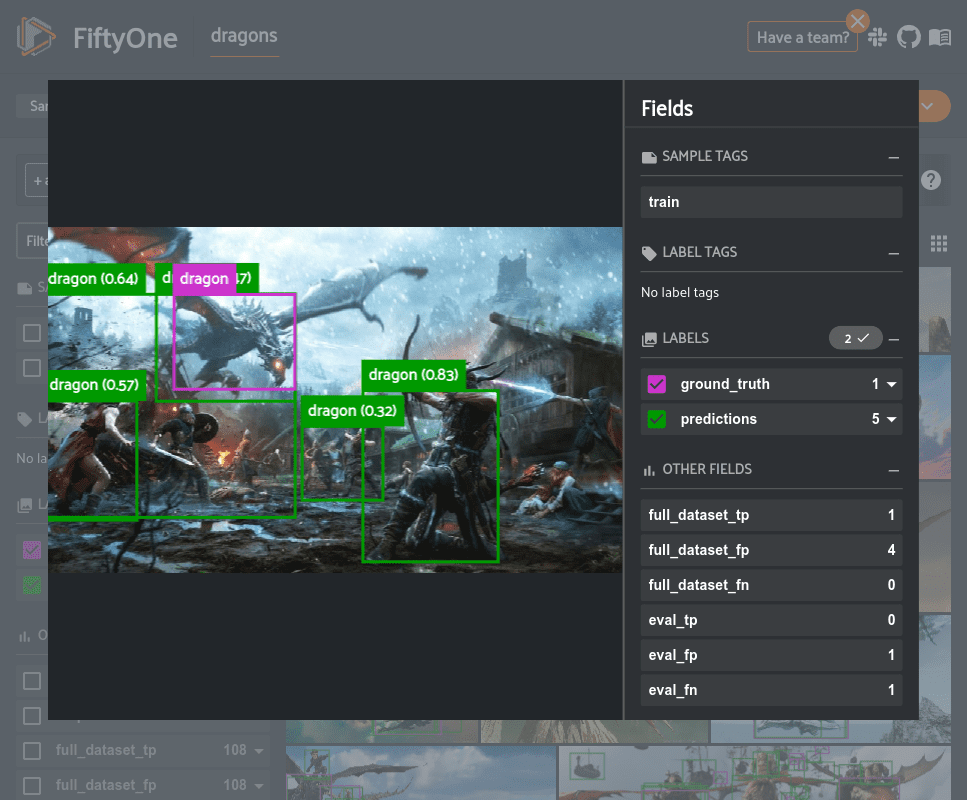
Now that the model predictions are loaded, we can dig in and analyze the results. FiftyOne provides methods for evaluating classification, detection, and segmentation models. While these methods can be used to compute dataset-wide metrics like so many other tools, the primary benefit is that this evaluation also populates instance-level results on the dataset like tagging individual true or false positive predictions. This allows you to not only understand how the model performs on the dataset as a whole but also specific instances in which the model performs well or poorly which is the best way to build intuition about the type of data you should use to retrain the model.

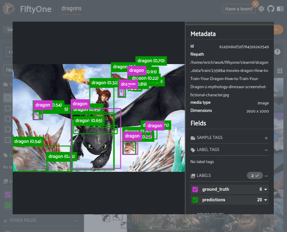
Visualizing predictions in FiftyOne shows many low confidence incorrect predictions. This indicates that we should find an appropriate confidence threshold to limit the predictions in the dataset.

One way to find a threshold value for detection confidence is to calculate the number of true and false positives that exist currently and find the point at which there are an equal number of both.

Let’s call the evalute_detections() method to use COCO-style object detection evaluation to compute if each ground truth and prediction is either a true positive, false positive, or false negative.

eval_key = "full_dataset_eval"
results = dataset.evaluate_detections(
  "predictions",
  gt_field="ground_truth",
  eval_key="full_data_eval",
)

The FiftyOne API provides a powerful query language that can be used to filter and slice datasets letting you look at the specific view in which you are interested. It also provides dataset-wide aggregation functions that let you easily access content from your datasets such as label values, counts, distributions, and ranges. One of these aggregations is the histogram_values() function that is perfect for our use case of computing the number of true and false positives for each confidence bin.

from fiftyone import ViewField as F
import numpy as np
import matplotlib.pyplot as plt

# Compute views of only True Positives and only False Positives
tp_view = dataset.filter_labels("predictions", F(eval_key) == "tp")
fp_view = dataset.filter_labels("predictions", F(eval_key) == "fp")

# Aggregate and plot histogram values
tp_counts, tp_edges, other = tp_view.histogram_values("predictions.detections.confidence", bins=50)
fp_counts, fp_edges, other = fp_view.histogram_values("predictions.detections.confidence", bins=50)

plt.plot(tp_edges[:-1][::-1], np.cumsum(tp_counts[::-1]))
plt.plot(fp_edges[:-1][::-1], np.cumsum(fp_counts[::-1]))
plt.show()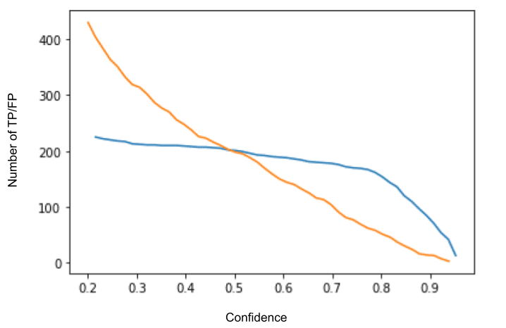

Based on this graph, we should set our confidence threshold to around 0.5. After browsing through the samples in the dataset, a threshold of 0.5 provides enough flexibility to detect many of the dragons in the dataset without too many false positives.

Now to apply this threshold and rerun evaluation to compute mAP.

high_conf_view = dataset.filter_labels(
  "predictions",
  F("confidence") > 0.5,
)
results = high_conf_view.evaluate_detections(
  "predictions",
  gt_field="ground_truth",
  eval_key="eval",
  compute_mAP=True,
)
print(results.mAP())
# 0.3417

What can our failures teach us?

One of the primary uses of FiftyOne is the ability to easily query and explore your dataset and model predictions for any question that comes to mind. An especially useful workflow is to explore the failure modes of your model to get a sense of how to best improve it going forward.

For example, let’s take a look at all of the predictions that were false positives but with high confidence, indicating that the model was fairly certain about its detection but was incorrect. These types of examples usually indicate either an ingrained issue with the model or an error in the ground truth annotations. Either need to be addressed promptly.

high_conf_fp = high_conf_view.filter_labels(
  "predictions",
  (F(eval_key) == "fp") & (F("confidence") > 0.9),
)

# Update App
session.view = high_conf_fp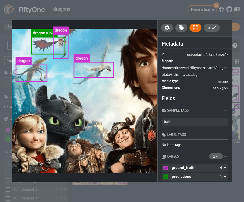

From the example above, it seems that one issue with our dataset is that we did not consistently annotate the wings of dragons. The model relatively accurately detected the dragon, but also included the wing which resulted in an IoU below the threshold used for evaluation (IoU=0.5). This detection would not necessarily be incorrect, though, so we may want to take a pass over the dataset to ensure dragon wings are consistently annotated. An easy way to reannotate this dataset is to use the integrations between FiftyOne and annotation tools like CVAT or Labelbox.

Now, let’s take a look at the false negatives in the dataset, where the model did not detect a ground truth object.

fn_view = high_conf_view.filter_labels(
  "ground_truth",
  F(eval_key) == "fn",
)

# Update App
session.view = fn_view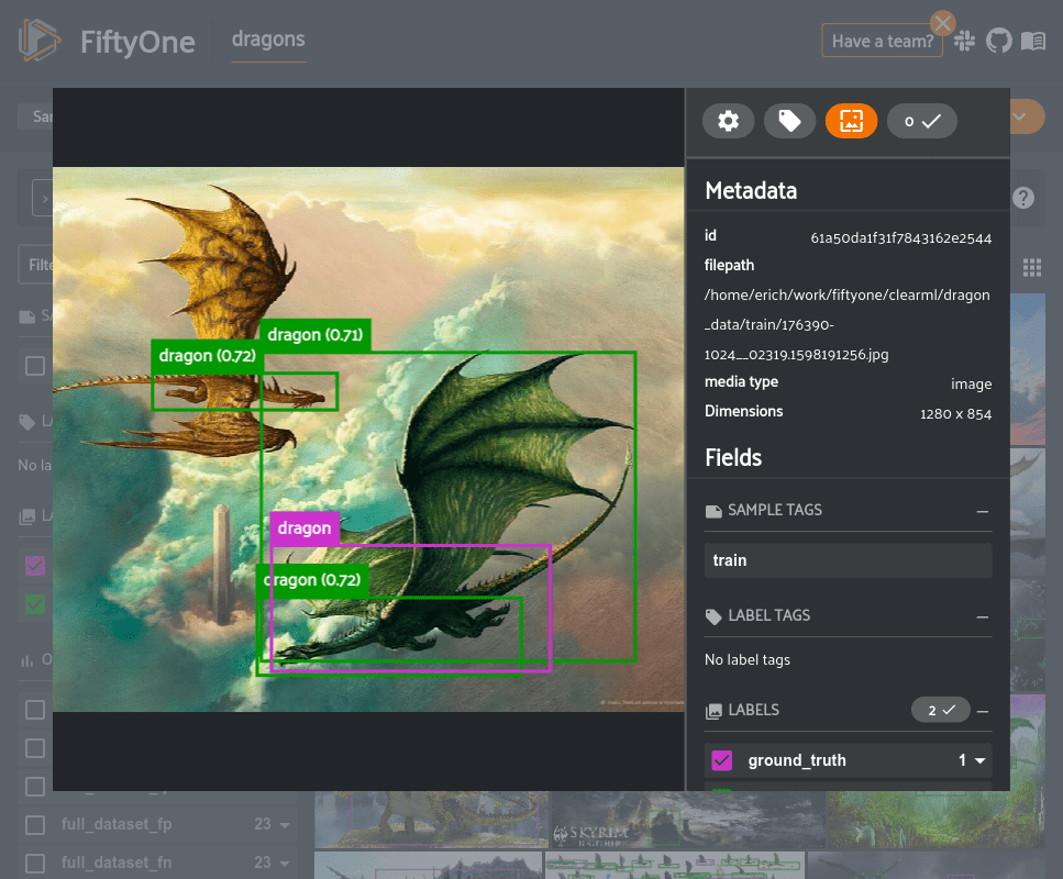

From the example above, we see another issue of the model incorrectly localizing the bounding box, even though it did detect the presence of a dragon. The comment about reannotating the dataset to include dragon wings still holds, however, it would also be useful to add additional training data to allow the model to learn to more accurately localize the boxes.

In the example above, we see that the model is frequently detecting non-dragon objects as dragons. The majority of the samples in this dataset contain only one or a few dragons isolated from other objects. Thus, the model seems to be learning to just detect all of the focal objects in the scene.

The best way to resolve this would be to add more scenes with multiple types of objects to the dataset as well as expand the classes to other object types so that the model is able to learn to better differentiate between dragons and other objects.

Next Steps

Based on the observations in the previous sections, we have a plan of action for producing a higher-quality dataset and a higher-performing model.

• Update the dataset annotations taking into account the wings
• Incorporate augmentations into the training loop
• Add more difficult samples like crowds of objects
• Automate and parameterize the training loop for fast retraining iterations whenever we update the data

Summary

Creating a high-performing model requires much more than just some PyTorch code. Being able to iteratively track and analyze model performance and then use that to inform dataset improvements is necessary for a high-quality model. The combination of the model analysis capabilities of FiftyOne with the experiment tracking capabilities of ClearML results in a system that will lead to better models, faster.

This post was made in collaboration between the teams at ClearML and Voxel51 and co-authored by Victor Sonck.