Using FiftyOne and Qdrant to generate classifications on your dataset utilizing model embeddings

Neural network embeddings are a low-dimensional representation of input data that give rise to a variety of applications. Embeddings have some interesting capabilities, as they are able to capture the semantics of the data points. This is especially useful for unstructured data like images and videos, so you can not only encode pixel similarities but also some more complex relationships.
Performing searches over these embeddings gives rise to a lot of use cases like classification, building up the recommendation systems, or even anomaly detection. One of the primary benefits of performing a nearest neighbor search on embeddings to accomplish these tasks is that there is no need to create a custom network for every new problem, you can often just use pre-trained models. In fact, it is possible to use the embeddings generated by some publicly available models without any further finetuning.
While there are a lot of powerful use cases that involve embeddings, there are a number of challenges in workflows performing searches over embeddings. Specifically, performing a nearest neighbor search on a large dataset and then being able to effectively act on the results of the search, for example performing workflows like auto-labeling of data, are both technical and tooling challenges. To that end, Qdrant and FiftyOne can help make these workflows effortless.
Qdrant is an open-source vector database designed to perform an approximate nearest neighbor search (ANN) on dense neural embeddings which is necessary for any production-ready system that is expected to scale to large amounts of data.
FiftyOne is an open-source dataset curation and model evaluation tool that allows you to effectively manage and visualize your dataset, generate embeddings, and improve your model results.
In this article, we’re going to load the MNIST dataset into FiftyOne and perform the classification based on ANN, so the data points will be classified by selecting the most common ground truth label among the K nearest points from our training dataset. In other words, for each test example, we’re going to select its K nearest neighbors, using a chosen distance function, and then just select the best label by voting. All that search in the vector space will be done with Qdrant, to speed things up. We will then evaluate the results of this classification in FiftyOne.
Installation
If you want to start using the semantic search with Qdrant, you need to run an instance of it, as this tool works in a client-server manner. The easiest way to do this is to use an official Docker image and start Qdrant with just a single command:
docker run -p “6333:6333” -p “6334:6334” -d qdrant/qdrant
After running the command we’ll have the Qdrant server running, with HTTP API exposed at port 6333 and gRPC interface at 6334.
We will also need to install a few Python packages. We’re going to use FiftyOne to visualize the data, along with their ground truth labels and the ones predicted by our embeddings similarity model. The embeddings will be created by MobileNet v2, available in torchvision. Of course, we need to communicate to Qdrant server somehow as well, and since we’re going to use Python, qdrant_client is a preferred way of doing that.
pip install fiftyone
pip install torchvision
pip install qdrant_client
Processing pipeline
- Loading the dataset
- Generating embeddings
- Loading embeddings into Qdrant
- Nearest neighbor classification
- Evaluation in FiftyOne
Loading the dataset
There are several steps we need to take to get things running smoothly. First of all, we need to load the MNIST dataset and extract the train examples from it, as we’re going to use them in our search operations. To make everything even faster, we’re not going to use all the examples, but just 2500 samples. We can use the FiftyOne Dataset Zoo to load the subset of MNIST we want in just one line of code.
import fiftyone as fo
import fiftyone.zoo as foz

# Load the data
dataset = foz.load_zoo_dataset("mnist", max_samples=2500)

# Get all training samples
train_view = dataset.match_tags(tags=["train"])
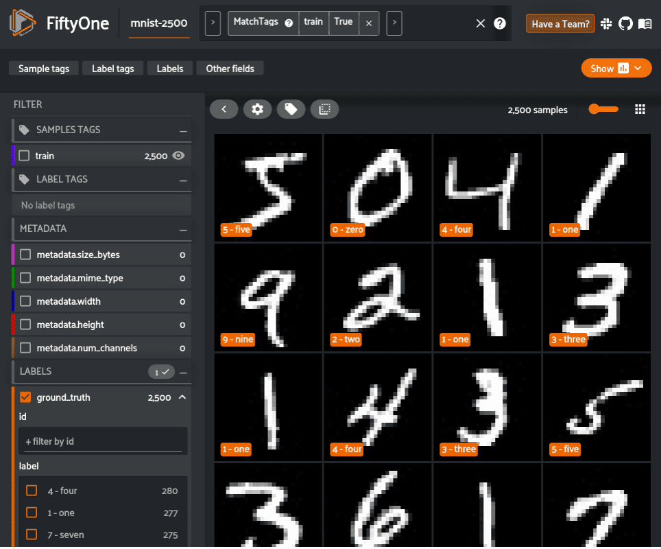
Let’s start by taking a look at the dataset in the FiftyOne App.
# Visualize the dataset in FiftyOne
session = fo.launch_app(train_view)
Generating embeddings
The next step is to generate embeddings on the samples in the dataset. This can always be done outside of FiftyOne, with your own custom models. However, FiftyOne also provides various different models in the FiftyOne Model Zoo that can be used right out of the box to generate embeddings.
In this example, we use MobileNetv2 trained on ImageNet to compute an embedding for each image.
# Compute embeddings
model = foz.load_zoo_model("mobilenet-v2-imagenet-torch")

train_embeddings = train_view.compute_embeddings(model)
Loading embeddings into Qdrant
Qdrant allows storing not only vectors but also some corresponding attributes — each data point has a related vector and optionally a JSON payload attached to it. We want to use this to pass in the ground truth label to make sure we can make our prediction later on.
ground_truth_labels = train_view.values("ground_truth.label")
train_payload = [
    {"ground_truth": gt} for gt in ground_truth_labels
]
Having the embedding created, we can simply start communicating with the Qdrant server. An instance of QdrantClient is then helpful, as it encloses all the required methods. Let’s connect and create a collection of points, simply called “mnist”. The vector size is dependent on the model output, so if we want to experiment with a different model another day, then we will just need to import a different one, but the rest will be kept the same. Eventually, after making sure the collection exists, we can send all the vectors along with their payloads containing their true labels.
import qdrant_client as qc
from qdrant_client.http.models import Distance, VectorParams

# Load the train embeddings into Qdrant
def create_and_upload_collection(
    embeddings, payload, collection_name="mnist"
):
    client = qc.QdrantClient(host="localhost")
    client.recreate_collection(
        collection_name=collection_name,
        vectors_config=VectorParams(
            size=embeddings.shape[1],
            distance=Distance.COSINE,
        )
    )
    client.upload_collection(
        collection_name=collection_name,
        vectors=embeddings,
        payload=payload,
    )
    return client

client = create_and_upload_collection(train_embeddings, train_payload)
Nearest neighbor classification
Now to perform inference on the dataset. We can create the embeddings for our test dataset, but just ignore the ground truth and try to find it out using ANN, then compare if both match. Let’s take one step at a time and start with creating the embeddings.
# Assign the labels to test embeddings by selecting
# the most common label among the neighbours of each sample
test_view = dataset.match_tags(tags=["test"])
test_embeddings = test_view.compute_embeddings(model)
Time for some magic. Let’s simply iterate through the test dataset’s samples and their corresponding embeddings, and use the search operation to find the 15 closest embeddings from the training set. We’ll also need to select the payloads, as they contain the ground truth labels which are required to find the most common label in the neighborhood of a particular point. Python’s Counter class will be helpful to avoid any boilerplate code. The most common label will be stored as an “ann_prediction” on each test sample in FiftyOne.
This is encompassed in the function below which takes an embedding vector as input, uses the Qdrant search capability to find the nearest neighbors to the test embedding, generates a class prediction, and returns a FiftyOne Classification object that we can store in our FiftyOne dataset.
import collections
from tqdm import tqdm

def generate_fiftyone_classification(
    embedding, collection_name="mnist"
):
    search_results = client.search(
        collection_name=collection_name,
        query_vector=embedding,
        with_payload=True,
        top=15,
    )
    # Count the occurrences of each class and select the most common label
    # with the confidence estimated as the number of occurrences of
    # the most common label divided by a total number of results.
    counter = collections.Counter(
        [point.payload["ground_truth"] for point in search_results]
    )
    predicted_class, occurences_num = counter.most_common(1)[0]
    confidence = occurences_num / sum(counter.values())
    prediction = fo.Classification(
        label=predicted_class, confidence=confidence
    )
    return prediction

predictions = []

# Call Qdrant to find the closest data points
for embedding in tqdm(test_embeddings):
    prediction = generate_fiftyone_classification(embedding)
    predictions.append(prediction)

test_view.set_values("ann_prediction", predictions)
By the way, we estimated the confidence by calculating the fraction of samples belonging to the most common label. That gives us an intuition of how sure we were while predicting the label for each case and can be used in FiftyOne to easily spot confusing examples.
Evaluation in FiftyOne
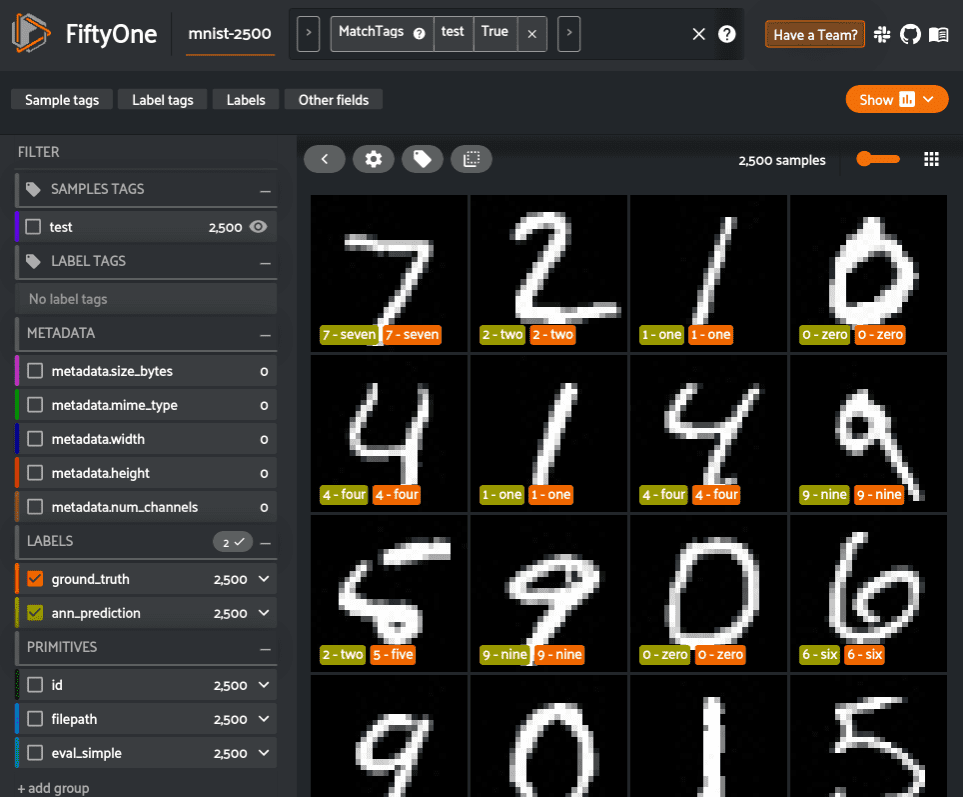
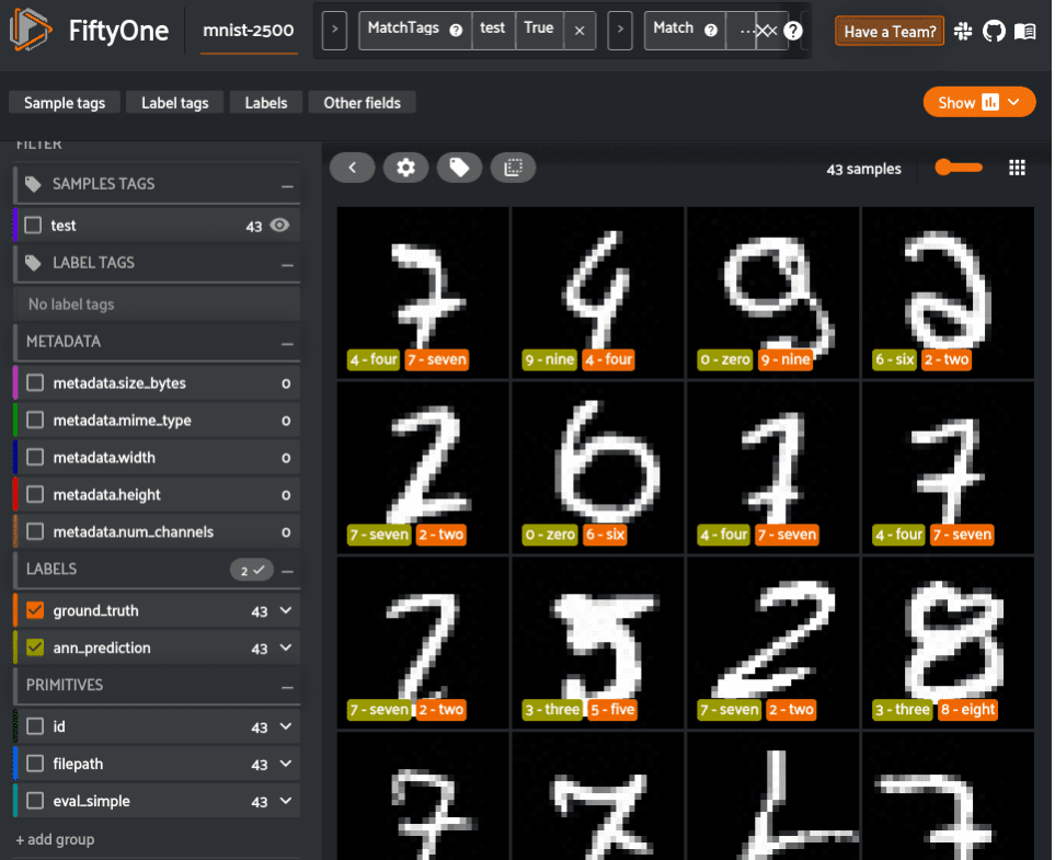
It’s high time for some results! Let’s start by visualizing how this classifier has performed. We can easily launch the FiftyOne App to view the ground truth, predictions, and images themselves.
session = fo.launch_app(test_view)
FiftyOne provides a variety of built-in methods for evaluating your model predictions, including regressions, classifications, detections, polygons, instance and semantic segmentations, on both image and video datasets. In two lines of code, we can compute and print an evaluation report of our classifier.
# Evaluate the ANN predictions, with respect to the values in ground_truth
results = test_view.evaluate_classifications(
    "ann_prediction", gt_field="ground_truth", eval_key="eval_simple"
)

# Display the classification metrics
results.print_report()
precision    recall  f1-score   support

    0 - zero       0.87      0.98      0.92       219
     1 - one       0.94      0.98      0.96       287
     2 - two       0.87      0.72      0.79       276
   3 - three       0.81      0.87      0.84       254
    4 - four       0.84      0.92      0.88       275
    5 - five       0.76      0.77      0.77       221
     6 - six       0.94      0.91      0.93       225
   7 - seven       0.83      0.81      0.82       257
   8 - eight       0.95      0.91      0.93       242
    9 - nine       0.94      0.87      0.90       244

    accuracy                           0.87      2500
   macro avg       0.88      0.87      0.87      2500
weighted avg       0.88      0.87      0.87      2500
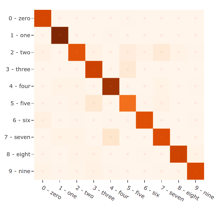
After performing the evaluation in FiftyOne, we can use the results object to generate an interactive confusion matrix allowing us to click on cells and automatically update the App to show the corresponding samples.
plot = results.plot_confusion_matrix()
plot.show()
Let’s dig in a bit further. We can use the sophisticated query language of FiftyOne to easily find all predictions that did not match the ground truth, yet were predicted with high confidence. These will generally be the most confusing samples for the dataset and the ones from which we can gather the most insight.
from fiftyone import ViewField as F

# Display FiftyOne app, but include only the wrong predictions that
# were predicted with high confidence
false_view = (
    test_view
    .match(F("eval_simple") == False)
    .filter_labels("ann_prediction", F("confidence") > 0.7)
)
session.view = false_view
These are the most confusing samples for the model and, as you can see, they are fairly irregular compared to other images in the dataset. A next step we could take to improve the performance of the model could be to use FiftyOne to curate additional samples similar to these. From there, those samples can then be annotated through the integrations between FiftyOne and tools like CVAT and Labelbox. Additionally, we could use some more vectors for training or just perform a fine-tuning of the model with similarity learning, for example using the triplet loss. But right now this example of using FiftyOne and Qdrant for vector similarity classification is working pretty well already.
And that’s it! As simple as that, we created an ANN classification model using FiftyOne with Qdrant as an embeddings backend, so finding the similarity between vectors can stop being a bottleneck as it would in the case of a traditional k-NN.
Try it yourself!
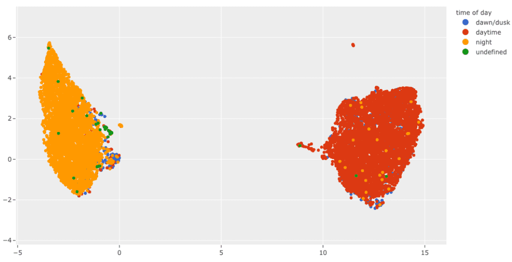
Click here for the notebook containing the source code of what you saw in this. Additionally, it includes a realistic use case of this process to perform pre-annotation of night and day attributes on the BDD100K road-scene dataset.
Summary
FiftyOne and Qdrant can be used together to efficiently perform a nearest neighbor search on embeddings and act on the results on your image and video datasets. The beauty of this process lies in its flexibility and repeatability. You can easily load additional ground truth labels for new fields into both FiftyOne and Qdrant and repeat this pre-annotation process using the existing embeddings. This can quickly cut down on annotation costs and result in higher-quality datasets, faster.
This blog post was made in collaboration between the teams at Qdrant and Voxel51 and is co-authored by Kacper Łukawski.

