Why notebooks have been great for CV/ML and what can still be learned from them.
FiftyOne, an open-source productivity for tool analyzing visual datasets, includes Jupyter notebook support, a feature which I implemented and was technical lead for. I set out to write an article describing the importance of such a feature — why automatic screenshotting is great for sharing your visual findings with others, why having code and its often visual outputs in one place has been so great for CV/ML, and how using FiftyOne in notebooks can unlock even more of the a paradigm established by notebooks for CV/ML engineers and researchers. This article hopes to do all of those things, but in its essence, it was also pulled in another direction as I learned the history of scientific notebooks. A history that begins with scientific research itself. And a history thematic of an openness that FiftyOne hopes to build upon.
So much more than Jupyter notebooks is needed by the CV/ML community for visual research and analysis.
The final section of this article is a step-by-step guide to using FiftyOne in notebooks to help you find problems with your visual datasets. The entire section can found in full via Google’s Colab, as well. We will see how to confirm a common failure mode of an image detection model and identify annotation mistakes, with very few lines of code, all while visualizing results each step of the way. But before that, indulge me in an attempt to explain why so much more than Jupyter notebooks is needed by the CV/ML community for visual research and analysis.
A Scientific State of Affairs
The collaborative efficiency of the scientific paper has reached a bottleneck.
In April of 2018, The Atlantic published an article declaring the obsolescence of the scientific paper as we know it. In truth, it may have merely been a willful prediction, or, in the least, shameless hyperbole for the internet to gobble up. But the history of scientific publishing it outlines is inarguable. The collaborative efficiency of the scientific paper has reached a bottleneck, nearly 400 years after its creation. The steady and incremental progress that was made by a “buzzing mass” of scientific researchers, to paraphrase the article, is now no longer suited for the times. Hundreds, perhaps even thousands, of researchers now publish in a field, not dozens. And results are often no longer computed by hand, but by computers, software, and datasets of once incomprehensible size.
Repeatability has become more important now than ever because of this scale. But often the steps taken to enable fellow researchers to reproduce one’s results are inadequate. All too often the code and data provided is incomplete, if it is provided at all, and complex ideas that are formulated using rich and dynamic visualizations are described with abstract language and reductive and static diagrams. The way in which research is shared no longer matches the way in which it is done.
Wolfram’s Walled Garden
The computational complexity and scale with which modern research is done has been a boon for scientific progress and technological innovation. Juxtaposed with the stubborn form of the scientific research paper (i.e. a PDF), it has also been an acknowledged problem for decades. A solution has been around for decades, though. A solution in which research is done and shared in the same way, the same form even. That solution was born as the computational “notebook” in 1988 when Wolfram Research, founded by Steven Wolfram, released Mathematica. Spearheaded by Theodore Gray, the interface was informed by an early Apple code editor, and in part formulated with help from none other than Steve Jobs.
For over thirty years Mathematica has continued to add to the number questions it can answer for you, the number ways you can visualize data, and the amount of data at your disposal. But growth has been slow since the first decade it was introduced. Licenses are expensive, publishers don’t want to use them, and what is supported in Mathematica starts and stops with Wolfram Research. It is a beautiful and incredibly capable walled garden.
Python, Jupyter, and So Much More
As Mathematica continued its march toward proprietary perfection, in early 2001 a graduate student in physics, Fernando Pérez, found himself fed up with his own ability to do research, even with Mathematica at his disposal. Per The Atlantic, he was enamored with the new programming language Python, and with the help of two other graduate students began a project that came to be known as IPython, the foundation of the Jupyter Project.
Jupyter has triumphed over Mathematica not along the “technical dimension”, but the “social dimension”.
Today, at the core of the Jupyter Project is the Jupyter Notebook. Like Mathematica, Jupyter Notebook encourages scientific exploration. But unlike Mathematica, it is an open-source project that anyone can contribute to. Similar to the “buzzing mass” of productivity that the scientific paper enabled neearly 400 years ago, Jupyter has triumphed over Mathematica not along the “technical dimension”, but the “social dimension” as Nobel Laureate Paul Romer noted. The form of Jupyter Notebooks is dictated by an active community of developers and users who have a stake in its success.
The field of computer vision stands firmly within the domain of scientific research. And for many years both academic and industry researchers have found incredible value in Jupyter Notebooks. Individual pieces of data are often the images and video themselves, and they need to be looked at and watched. Notebooks offer that. Reproducible visualizations need to be shared. Notebooks offer that. And the open ecosystem of Jupyter allows for any missing integration to be easily added.
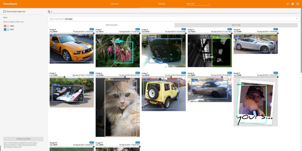
Packages like matplotlib and opencv can be used to display images and video that need to be inspected. When training machine learning models, packages like tensorboard offer sample visualizations that extend inspection of images into the context of experiment tracking. matplotlib, opencv, tensorboard, and countless other Python packages with visualization capabilities can all be seamlessly used within Jupyter Notebooks.
Understanding data quality requires an informed sense of the trends in one’s data.
Though, in CV/ML, a stark issue remains when using Jupyter notebooks. Data quality is critical to building great models. And understanding data quality requires an informed sense of the trends in one’s data. Looking at one or even a dozen images is almost always not enough to understand the performance and failure modes of a model. Furthermore, identifying individual mistakes in ground truth or gold standard labels that may only occur in one out of 1,000 or even 100,000 images requires rapid slicing and dicing of datasets to narrow in on problems. Fundamentally, there is a lack of tooling available for naturally working with visual datasets in notebooks that allows for this kind of problem solving.
FiftyOne and Jupyter
So, “What is FiftyOne?”. It is an open-source CV/ML project that hopes to solve many of the practical problems and tooling problems faced by CV/ML researchers in industry and academia. It is the reason I am writing this article, and the reason why I think the history of computational notebooks contains valuable lessons. As a developer of FiftyOne, I admire the quality of research that it encourages, and the collaboration it allows for. And I agree that progress is often best made in an open, sometimes noisy, forum.
The opportunity to have machines make intelligent and automated decisions for us has prompted a massive manual undertaking.
The brief history of notebooks and scientific publishing outlined earlier serve as a parallel to the many problems facing machine learning today. Specifically, in the domain of computer vision. Computer visions models attempt to make observations and decisions about unstructured, human-made, artifacts of our world, i.e. images and video. Large datasets numbering in the millions of images have been imperfectly annotated by thousands of workers in the past decade in pursuit of training and understanding the performance of theses models. The opportunity to have machines make intelligent and automated decisions for us has prompted a massive manual undertaking. Ironic, to say the least.
Recent efforts in more unsupervised approaches to computer vision tasks that do not require the arduous and costly work of human annotation such as OpenAI’s CLIP have proven to be fruitful. But performance still remains far from perfect. And, in the very least, understanding model performance will always require manual verification against trusted, ground truth or gold standard data. Or at least it should. After all, these models are not being sent off into the woods to operate and infer among themselves. Models are being embedded into our everyday life, and the quality of their performance can have life and death consequences.
The quality of methods and tools we use to analyze computer vision models should match, if not exceed, the quality of methods and tools used to build them.
It stands, therefore, that the quality of methods and tools we use to analyze computer vision models should match, if not exceed, the quality of methods and tools used to build them. And that cumulative, collaborative, and incremental problem solving is paramount. Establishing open standards that enable the CV/ML community to work together, incrementally, as a “buzzing mass” not just on models, but on datasets is likely the only tractable way to establish trust and progress in the science of modern computer vision. FiftyOne hopes to enable this establishment of trust and progress.
What follows is a small example of the current capabilities of FiftyOne, focused on demonstrating the foundational APIs and UX that allow one to answer questions they have about their datasets and models efficiently, all within a Jupyter notebook.
Digging Into COCO, with FiftyOne
Follow along in this Colab notebook!
Notebooks offer a convenient way to analyze visual datasets. Code and visualizations can live in the same place, which is exactly what CV/ML often requires. With that in mind, being able to find problems in visual datasets is the first step towards improving them. This section walks us though each “step” (i.e., a notebook cell) of digging for problems in an image dataset. I encourage you to click through to the Colab notebook and experience the journey yourself. First, we’ll need to install the fiftyone package with pip.
pip install fiftyone
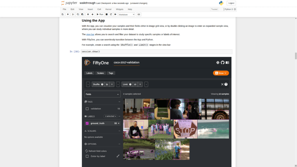
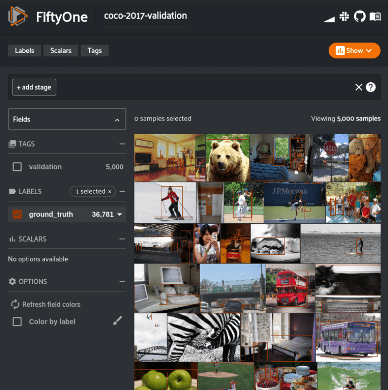
Next, we can download and load our dataset. We will be using the COCO-2017 validation split. Let’s also take a moment to visualize the ground truth detection labels using the FiftyOne App. The following code will do all of this for us.
import fiftyone as fo
import fiftyone.zoo as foz

dataset = foz.load_zoo_dataset("coco-2017", split="validation")
session = fo.launch_app(dataset)
We have our COCO-2017 validation dataset loaded, now let’s download and load our model and apply it to our validation dataset. We will be using the faster-rcnn-resnet50-fpn-coco-torch pre-trained model from the FiftyOne Model Zoo. Let’s apply the predictions to a new label field predictions, and limit the application to detections with a confidence greater than or equal to 0.6.
model = foz.load_zoo_model("faster-rcnn-resnet50-fpn-coco-torch")
dataset.apply_model(model, label_field="predictions", confidence_thresh=0.6)
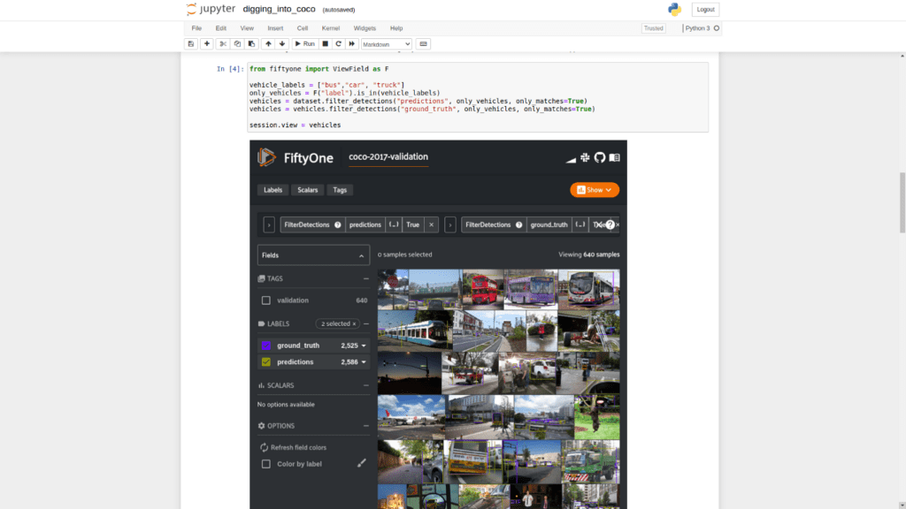
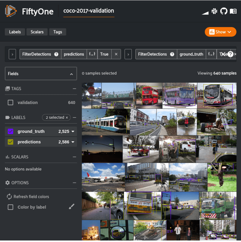
Let’s focus on issues related vehicle detections and consider all buses, cars, and trucks vehicles and ignore any other detections, in both the ground truth labels and our predictions.
The following filters our dataset to a view containing only our vehicle detections, and renders the view in the App.
from fiftyone import ViewField as F

vehicle_labels = ["bus","car", "truck"]
only_vehicles = F("label").is_in(vehicle_labels)

vehicles = (
    dataset
    .filter_labels("predictions", only_vehicles, only_matches=True)
    .filter_labels("ground_truth", only_vehicles, only_matches=True)
)

session.view = vehicles
Now that we have our predictions, we can evaluate the model. We’ll use an evaluate_detections() utility method provided by FiftyOne that uses the COCO evaluation methodology.
from fiftyone.utils.eval import evaluate_detections

evaluate_detections(vehicles, "predictions",  gt_field="ground_truth", iou=0.75)
evaluate_detections() has populated various pieces of data about the evaluation into our dataset. Of note is information about which predictions were not matched with a ground truth box. The following view into the dataset lets us look at only those unmatched predictions. We’ll sort by confidence, as well, in descending order.
filter_vehicles = F("ground_truth_eval.matches.0_75.gt_id") == -1

unmatched_vehicles = (
    vehicles
    .filter_labels("predictions", filter_vehicles, only_matches=True)
    .sort_by(F("predictions.detections").map(F("confidence")).max(), reverse=True)
)

session.view = unmatched_vehicles
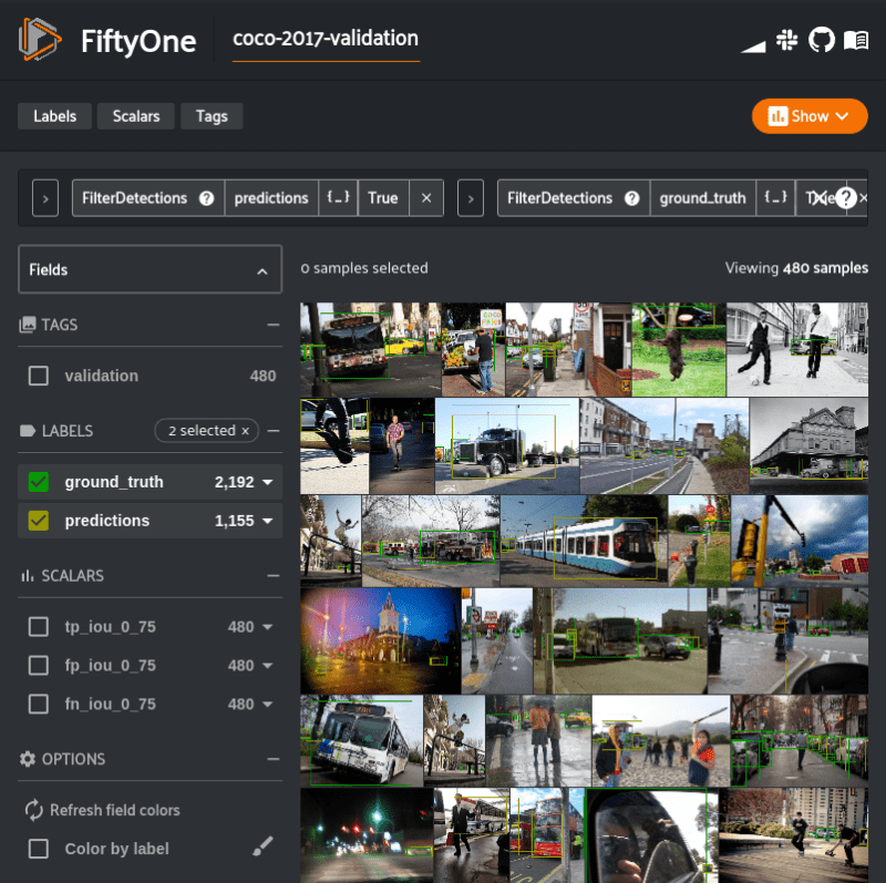
If you were working in a notebook version of this walk through, you would see that the most common reason for an unmatched prediction is that there is a label mismatch. It is not surprising, as all three of these classes are in the vehicle supercategory. Trucks and cars are often confused in human annotation and model prediction.
Looking beyond class confusion, though, let’s take a look at the first two samples in our unmatched predictions view.

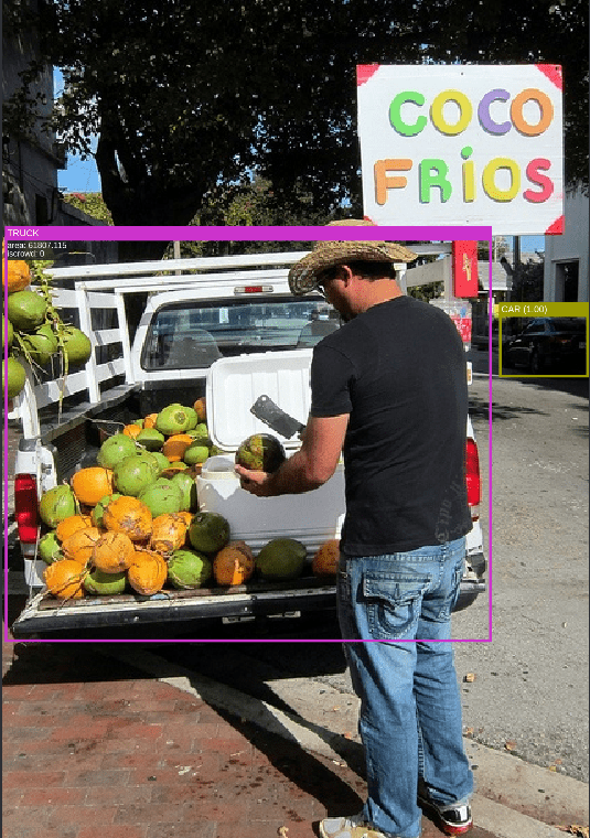
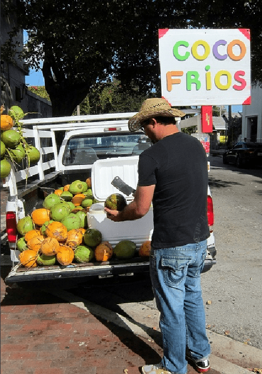
The very first sample, found in the pictures above, has an annotation mistake. The truncated car in the right of the image has too small of a ground truth bounding box (pink). The unmatched prediction (yellow) is far more accurate, but did not meet the IoU threshold.
 |
 |
|||
The predicted box of the car in the shadow of the trees is correct, but it is not labeled in the ground truth. Raw image from the COCO 2017 detection dataset. (Images by author) |
||||
The second sample found in our unmatched predictions view contains a different kind of annotation error. A more egregious one, in fact. The correctly predicted bounding box (yellow) in the image has no corresponding ground truth. The car in the shade of the trees was simply not annotated.
Manually fixing these mistakes is out of the scope of this example, as it requires a large feedback loop. FiftyOne is dedicated to making that feedback loop possible (and efficient), but for now let’s focus on how we can answer questions about model performance, and confirm the hypothesis that our model does in fact confuse buses, cars, and trucks quite often.
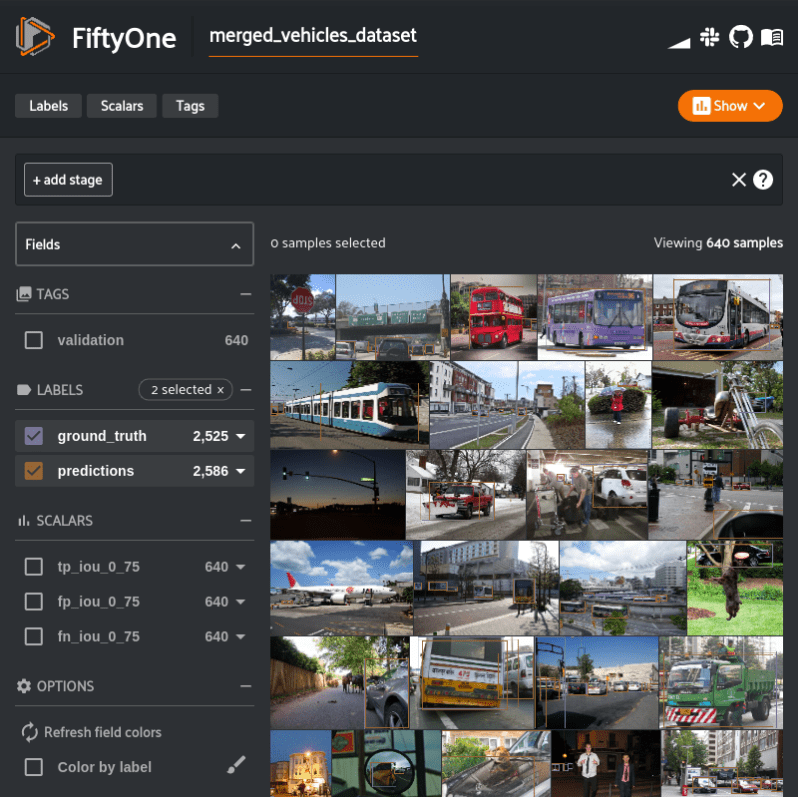
We’ll do this by reevaluating our predictions with buses, cars, and trucks all merged into a single vehicle label. The following creates such a view, clones the view into a separate dataset so we’ll have separate evaluation results, and evaluates the merged labels.
vehicle_labels = {
    label: "vehicle" for label in ["bus","car", "truck"]
}

merged_vehicles_dataset = (
    vehicles
    .map_labels("ground_truth", vehicle_labels)
    .map_labels("predictions", vehicle_labels)
    .exclude_fields(["tp_iou_0_75", "fp_iou_0_75", "fn_iou_0_75"])
    .clone("merged_vehicles_dataset")
)

evaluate_detections(
    merged_vehicles_dataset, "predictions", gt_field="ground_truth", iou=0.75)

session.dataset = merged_vehicles_dataset
Now we have evaluation results for the originally segmented bus, car, and truck detections and the merged detections. We can now simply compare the number of true positives from the original evaluation, to the number of true positives in the merged evaluation.
original_tp_count = vehicles.sum("tp_iou_0_75")
merged_tp_count = merged_vehicles_dataset.sum("tp_iou_0_75")

print("Original Vehicles True Positives: %d" % original_tp_count)
print("Merged Vehicles True Positives: %d" % merged_tp_count)
We can see that before merging the bus, car, and truck labels there were 1,431 true positives. Merging the three labels together resulted in 1,515 true positives.
Original Vehicles True Positives: 1431
Merged Vehicles True Positives: 1515
We were able to confirm our hypothesis! Albeit, a quite obvious one. But we now have a data-backed understanding a common failure mode of this model. And now this entire experiment can be shared with others. In a notebook, the following will screenshot the last active App window, so all outputs can be statically viewed by others.
session.freeze() # Screenshot the active App window for sharing
Summary
Notebooks have emerged as a popular medium for performing and sharing data science, especially in the field of computer vision. But working with visual datasets has historically been a challenge, a challenge we hope to address with an open tool like FiftyOne. The notebook revolution is largely still in its infancy and will continue to evolve and become an even more compelling tool for performing and communicating ML projects in the community, hopefully, in part, because of FiftyOne!
Thanks for following along! The FiftyOne project can be found on GitHub. If you agree that the CV/ML community needs an open tool to solve its data problems, give us a star!

