Finding Images with Words

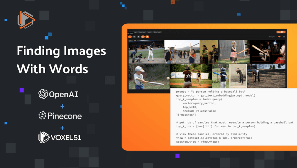
Add natural language image search to your computer vision pipelines with FiftyOne, Pinecone, and CLIP

One of the coolest things to happen in machine learning over the past few years is the dramatic improvement of multi-modal AI , and the ensuing cross-pollination between computer vision and natural language processing. At the center of this movement is OpenAI’s CLIP model, which uses a contrastive learning technique to embed multimedia content — in this case language and images — into the same latent space.

The quality of multi-modal models like CLIP has led to advances in zero-shot image classification, knowledge transfer, synthetic data generation, and semantic search. It is the last of these that we will be focusing on today!

While you may have seen standalone vector search tools, libraries, or demonstrations, today we’re going to show you how to incorporate natural language image search directly into your computer vision workflows. To do this, we will be making use of the open source computer vision toolkit FiftyOne, vector database Pinecone, and OpenAI’s CLIP model.

In this article, we’ll cover:

• Loading in your data and embedding model
• Generating CLIP embeddings
• Creating a vector index
• Querying your vector index with text prompts
• What you can use this for!

Read on to learn how to move beyond labels and towards more general understanding of your computer vision data!

Getting set up

The first thing we need to do is install the relevant packages.

# install FiftyOne
pip install fiftyone

# install Pinecone
pip install -U pinecone-client

Once FiftyOne is installed, we are good to go, and we can import the library. We’ll also import the fiftyone.zoo submodule so we can quickly load in a subset of the MS COCO dataset from the FiftyOne Dataset Zoo, as well as a PyTorch implementation of the CLIP model from the FiftyOne Model Zoo:

import fiftyone as fo
import fiftyone.zoo as foz

dataset = foz.load_zoo_dataset("coco-2017", split="validation")
model = foz.load_zoo_model("clip-vit-base32-torch")

If you’d like, you can instead download OpenAI’s CLIP model directly from source by following instructions here.

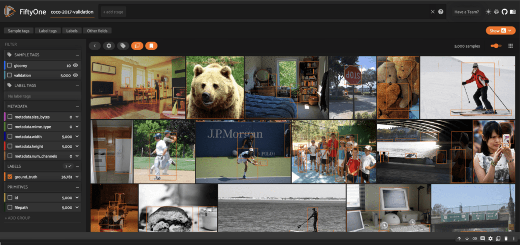
Before setting up Pinecone, we can take a look at our data in the FiftyOne App, which you can instantiate in your browser, within a Jupyter notebook, or as a standalone desktop application:

session = fo.launch_app(dataset)

To get started working with Pinecone, you need to set up an account here, if you don’t have one already, and copy an API key from here. Import Pinecone and pass in an API key as follows:

import pinecone

pinecone.init(api_key="API-KEY", environment="us-west1-gcp")

Finally, we’ll import the remaining packages that we will need, and will configuring our PyTorch data type:

import numpy as np
from pkg_resources import packaging
import torch

device = "cuda" if torch.cuda.is_available() else "cpu"

if packaging.version.parse(
  torch.__version__
) < packaging.version.parse("1.8.0"):
  dtype = torch.long
else:
  dtype = torch.int

Generating CLIP embeddings

To perform searches on our images based on text prompts, we need to generate embeddings for both the images in our dataset, and any text prompts we might want to search against.

With FiftyOne’s compute_embeddings() method, we can generate embeddings for all of the images in our dataset in one fell swoop, storing them in an embedding field:

dataset.compute_embeddings(
    model, 
    embeddings_field="embedding"
)

This might take a few minutes, as computing embeddings from deep neural models is in general a relatively intensive task. If you plan to generate embeddings for many samples, best practice is to pre-compute them ahead of time, and if you intend to use these embeddings more than once, I suggest you persist this data by setting

dataset.persistent = True

If we’d like, we can also pair these embeddings with a dimensionality reduction technique to visualize the embeddings. Using the FiftyOne Brain, we can do this with the compute_visualization() method:

import fiftyone.brain as fob
from fiftyone import ViewField as F

# perform dimensionality reduction using t-SNE
results = fob.compute_visualization(
    dataset, 
    embeddings = "embedding", 
    method = "tsne"
)

# visualize results, labeling by number of objects in image
results.visualize(labels=F("ground_truth.detections").length())

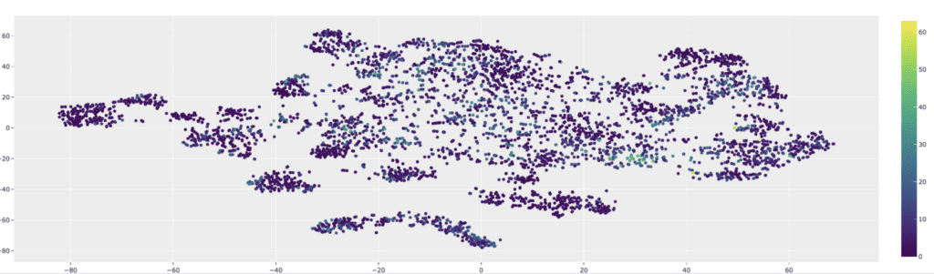
Even in this very basic visualization, we can see that the images with tons of objects tend to cluster together. There’s much more that can be gleaned from visualizations like this, but that is not the focus of this article.

To compute the embedding for a text prompt, we need to first tokenize the text, then generate a feature vector for the input text which standardizes format, and finally encode this feature vector. The following function takes in a text prompt and the FiftyOne-wrapped PyTorch CLIP model we loaded, and performs the logic of generating the corresponding embedding vector:

def get_text_embedding(prompt, clip_model):
    tokenizer = clip_model._tokenizer

    # standard start-of-text token
    sot_token = tokenizer.encoder["<|startoftext|>"]

    # standard end-of-text token
    eot_token = tokenizer.encoder["<|endoftext|>"]

    prompt_tokens = tokenizer.encode(prompt)
    all_tokens = [[sot_token] + prompt_tokens + [eot_token]]

    text_features = torch.zeros(
        len(all_tokens),
        clip_model.config.context_length,
        dtype=dtype,
        device=device,
    )

    # insert tokens into feature vector
    text_features[0, : len(all_tokens[0])] = torch.tensor(all_tokens)

    # encode text
    embedding = clip_model._model.encode_text(text_features).to(device)

    # convert to list for Pinecone
    return embedding.tolist()

To generate the embedding for the prompt “a picture of a giraffe”, we could do so with

prompt = "a picture of a giraffe"
query_vector = get_text_embedding(prompt, model)

Creating the vector index

If you have a paid Pinecone account, then you can work with multiple vector indices at once. However, for this article we’ll be assuming only a free Pinecone account, which limits you to one vector index. In this case, you should run the following code block to delete any existing vector index associated with your account before creating a new one.

indices = pinecone.list_indexes()
if len(indices) > 0:
    pinecone.delete_index(indices[0])

After doing so, you can create a new vector index:

index_name = "my-index"
pinecone.create_index(
    index_name, 
    dimension=512, 
    metric="cosine", 
    pod_type="p1"
)
index = pinecone.Index(index_name)

Here we have named the index “my-index” for illustrative purposes, but you can use whatever name you would like. We’ve passed in dimension=512 because that is the dimension of the embedding vectors generated by CLIP, and we have chosen to use a "cosine" metric — vectors will be indexed according to their cosine similarity to the query vector. Of course, in general the use of metrics like cosine similarity only makes sense if the embedding vectors have been properly normalized. The pod_type="p1" refers to the hardware running the Pinecone service; p1 pods support up to one million vectors.

Now we populate the vector database with the embedding vectors from our dataset, upserting 100 vectors at a time:

# convert numpy arrays to lists for pinecone
embeddings = [arr.tolist() for arr in dataset.values("embedding")]
ids = dataset.values("id")

# create tuples of (id, embedding) for each sample
index_vectors = list(zip(ids, embeddings))

def upsert_vectors(index, vectors):
    num_vectors = len(vectors)
    num_vectors_per_step = 100
    num_steps = int(np.ceil(num_vectors/num_vectors_per_step))
    for i in range(num_steps):
        min_ind = num_vectors_per_step * i
        max_ind = min(num_vectors_per_step * (i+1), num_vectors)
        index.upsert(index_vectors[min_ind:max_ind])

upsert_vectors(index, index_vectors)

One subtle note is that we are using FiftyOne’s "id" value to identify these embedding vectors. We do this because all "id" identifiers are unique in FiftyOne, and we can index or subset the samples in our dataset by passing in a list of these values, as we will do shortly.

Querying the dataset

Now that we have a vector index and a function for computing the embedding vector for an input text prompt, we are ready to query on our data.

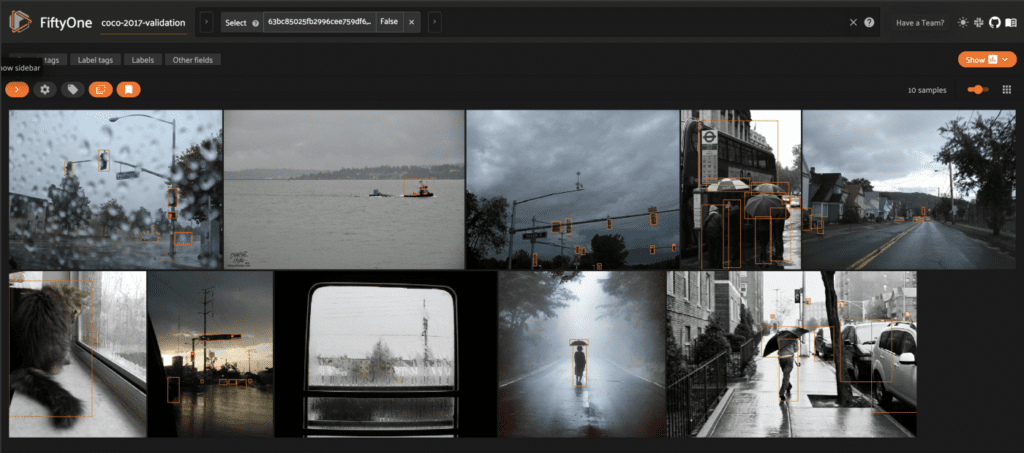
To start, let’s say we want to find the 10 gloomiest images. We can do this by first generating the query vector:

prompt = "a gloomy day"
query_vector = get_text_embedding(prompt, model)

Then querying our vector index for the 10 most similar embedding vectors top_k=10 to this query vector:

top_k_samples = index.query(
    vector=query_vector,
    top_k=10,
    include_values=False
)['matches']

This returns a list of (ten) results, sorted by `score` on the cosine similarity metric.

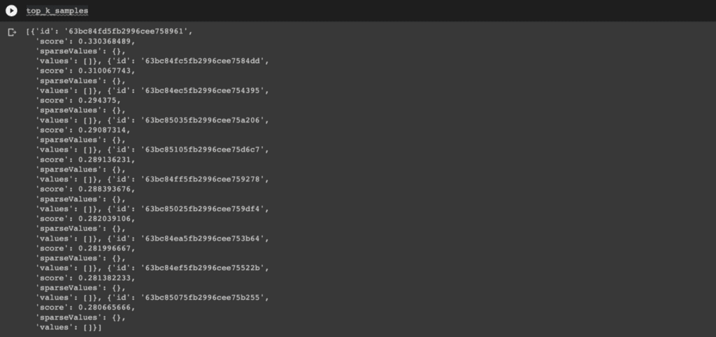
Because cosine is a similarity metric and not a distance metric, the most similar results have the highest scores. If you used the “euclidean” distance metric instead, the most similar results would be those with scores closest to zero.

Finally, we can use these results to generate a view of the associated samples in FiftyOne. If we wanted to, we could save and store the score values generated by this query in a field on the samples. For this illustration however, we’ll keep it simple:

# get ids of gloomiest samples
top_k_ids = [res['id'] for res in top_k_samples]

# view these samples, ordered by “gloominess”
view = dataset.select(top_k_ids, ordered=True)
session.view = view.view()

We could also query for more complicated things, like “a person holding a baseball bat”:

prompt = "a person holding a baseball bat"
query_vector = get_text_embedding(prompt, model)
top_k_samples = index.query(
    vector=query_vector,
    top_k=10,
    include_values=False
)['matches']

# get ids of samples that most resemble a person holding a baseball bat
top_k_ids = [res['id'] for res in top_k_samples]

# view these samples, ordered by similarity
view = dataset.select(top_k_ids, ordered=True)
session.view = view.view()

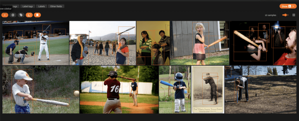
While the results aren’t perfect, it’s pretty amazing that you can write an arbitrary natural language query, run it on any arbitrary dataset, and achieve this level of performance and understanding. Just take a second and think about this. The fact that we don’t have to gather a dataset and train a classifier for this task is very cool, and very powerful!

Of course, it’s worth noting that results from using CLIP or another foundational multi-modal ML model out of the box like this will in all likelihood not beat a classifier trained or fine-tuned on your specific data for your specific task. But that is not the point.

This is an incredible tool to use for completely unsupervised and unstructured exploration of a new dataset!

At this point, we could tag these samples in Python for labeling or annotation:

view.tag_samples("possibly holding baseball bat")

Or you can use FiftyOne’s in-App tagging features.

Putting the pieces together

Now that we have seen the full workflow for querying our data with a search vector, let’s put it all together and wrap it in a function. We’ll call it sort_by_semantic_similarity(), drawing inspiration from the FiftyOne Brain method sort_by_similarity().

Let’s make it flexible enough to return either all samples, sorted by semantic similarity, or just the k most similar.

Note: the top_k argument for Pinecone queries is capped at 10000. We’ll also give an optional score_field argument where if score_field!= None, we will store the score values returned by the index query on the samples.

def sort_by_semantic_similarity(
    dataset,
    index,
    prompt,
    k=None,
    score_field=None
):
    
    query_vector = get_text_embedding(prompt, model)
    if k is not None:
        top_k=k
    else:
        top_k = int(min(10000, dataset.count()))
        
    
    result_samples = index.query(
        vector=query_vector,
        top_k=top_k,
        include_values=False
    )['matches']
    
    sample_ids = [res['id'] for res in result_samples]
    view = dataset.select(sample_ids, ordered=True)

    if score_field is not None:
        scores = [res['score'] for res in result_samples]
        dataset.add_sample_field(score_field, fo.FloatField)
        view.set_values(score_field, scores)
        dataset.save()
    
    return view

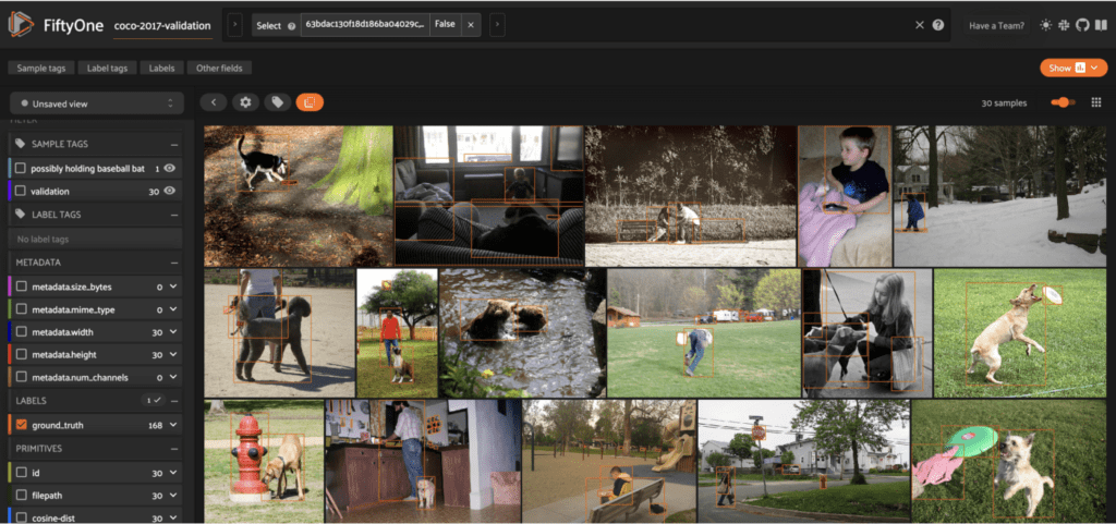
Let’s try it out:

prompt = "a child playing with a dog"

view = sort_by_semantic_similarity(
    dataset, 
    index, 
    prompt, 
    k = 30, 
    score_field = "cosine-dist"
)

session.view = view.view()

What can you use this for?

The ability to semantically search through your computer vision datasets can be immensely useful. You can use these capabilities to pre-annotate your data, or tag samples to send back to your labeling service provider for re-annotation. By setting a cutoff, you can also take advantage of the raw score values returned by the vector index query for zero-shot image classification or multi-output classification, or use it as a performance baseline while prototyping.

Perhaps most importantly, performing natural language image search using an off-the-shelf foundation model like CLIP can be a great way to perform ad hoc exploration of datasets in an unstructured way. You can query the data with any prompt you can possibly imagine, without the need to perform any model training or fine-tuning of any kind in order to get started. This can be useful in situations where you do not require an exhaustive or exact list of every sample that matches a given criteria. Maybe you are just interested in retrieving a few representative examples of a particular query. Or maybe you are interested in understanding the range of samples in your dataset, beyond aggregate statistics.

If you need more systematic results, you’ll likely need to have the data annotated, train or fine-tune a model, or otherwise pass your data on for further processing and analysis. But using CLIP (or another multi-modal embedding model) can help you begin to bootstrap these processes!

Conclusion

Whether you are building predictive models, looking for trends, or assessing the quality of your computer vision data, semantic search is a tool that every machine learning engineer or researcher should have in their arsenal. I hope this article has given you what you need to use this tool in your current and future computer vision workflows!

If you want to dive deeper, here are some things for you to play around with:

• Metrics: cosine vs euclidean…
• Embedding models: CLIP is not the only one!
• Vector search engines: Pinecone is just one of many options
• Prompt-crafting: how does the phrasing of the text prompt affect the result?

Join the FiftyOne community!

Join the thousands of engineers and data scientists already using FiftyOne to solve some of the most challenging problems in computer vision today!

• 1,250+ FiftyOne Slack members
• 2,400+ stars on GitHub
• 2,500+ Meetup members
• Used by 220+ repositories
• 54+ contributors