Editor’s note – This is the first article in the three-part series:
- Part 1 – Generate, load, and visualize YOLOv8 model predictions (this article)
- Part 2 – Evaluate YOLOv8 model predictions
- Part 3 – Fine-tune YOLOv8 models for custom computer vision applications
Generate, load, and visualize YOLOv8 model predictions
Welcome to the first part in our three part series on YOLOv8! In this series, we’ll show you how to work with YOLOv8, from downloading the off-the-shelf models, to fine-tuning these models for specific use cases, and everything in between.
Throughout the series, we will be using two libraries: FiftyOne, the open source computer vision toolkit, and Ultralytics, the library that will give us access to YOLOv8.
In Part 1, you’ll learn how to generate, load, and visualize YOLOv8 predictions. In Part 2, we’ll show you how to evaluate the quality of YOLOv8 model predictions. In Part 3, we’ll conclude by walking you through the process of fine-tuning YOLOv8 for your computer vision applications.
This post is organized as follows:
- YOLO family history
- Getting set up with YOLOv8
- Generating YOLOv8 predictions
- Visualizing YOLOv8 predictions with the FiftyOne App
Continue reading to learn how you can leverage FiftyOne to take a deeper look into YOLOv8’s predictions!
Background on YOLO models
Since its initial release back in 2015, the You Only Look Once (YOLO) family of computer vision models has been one of the most popular in the field. The core innovation of the YOLO architecture was to treat object detection tasks as regression problems, so that the model generates predictions for all object bounding boxes and class probabilities at the same time.
This approach represented a major shift from prior state of the art object detection models, wherein each detected object presented an increased inference load – hence the You Only Look Once, or YOLO moniker. And by streamlining the prediction pipeline, YOLO drastically reduced the inference time. The original YOLO model was able to process 45 frames per second!
Over the past eight years, this architectural innovation has spawned a family of YOLO models, each generation bringing improvements in speed and accuracy. The models were trained on new datasets. The architecture was extended to new domains like bird’s eye views. And the end-to-end detector was used in more and more applications.
In late 2022, Ultralytics announced the latest member of the YOLO family, YOLOv8, which comes with a new backbone. The “model” is actually a suite of models for object detection and instance segmentation. The suite includes models of various sizes, from 3.2 million parameters up to 68.2 million parameters, which achieve state of the art performance and retain the speed of their progenitors.
With YOLOv8, however, the basic detection and segmentation models are general purpose, which means for custom use cases they may not be suitable out of the box.
In this series, we’ll show you how to take a deeper look into YOLOv8’s predictions, and then use these insights to fine-tune the model for your own applications.
Getting started
If you haven’t already done so, install the Ultralytics and FiftyOne Python packages:
pip install fiftyone ultralytics
We will also import all of the other relevant Python packages:
import numpy as np
import os
from tqdm import tqdm
Next, we’ll import the relevant modules from FiftyOne. The base FiftyOne library will allow us to efficiently work with our computer vision data. We will use the FiftyOne Dataset Zoo to load subsets of the MS COCO dataset. And the ViewField will allow us to symbolically filter the data in our dataset.
import fiftyone as fo
import fiftyone.zoo as foz
from fiftyone import ViewField as F
Finally, we can import the YOLO object from Ultralytics and use this to instantiate pretrained detection and segmentation models in Python. Along with the YOLOv8 architecture, Ultralytics released a set of pretrained models, with different sizes, for classification, detection, and segmentation tasks.
For the purposes of illustration, we will use the smallest version, YOLOv8 Nano (YOLOv8n), but the same syntax will work for any of the pretrained models on the Ultralytics YOLOv8 GitHub repo.
from ultralytics import YOLO
detection_model = YOLO("yolov8n.pt")
seg_model = YOLO("yolov8n-seg.pt")
In this blog post series, we will call YOLOv8 models from the command line a majority of the time. However, as an illustration, we show how to use these models within a Python environment.
In Python, you can apply a YOLOv8 model to an individual image by passing the file path into the model call. For an image with file path path/to/image.jpg, running
detection_model("path/to/image.jpg")
will generate a list containing a single ultralytics.yolo.engine.results.Results object. A similar result can be obtained if we apply the segmentation model to an image. These results contain bounding boxes, class confidence scores, and integers representing class labels. For a complete discussion of these results objects, see the Ultralytics YOLOv8 Results API Reference.
If we want to run tasks on all images in a directory, then we can do so from the command line with the YOLO Command Line Interface by specifying the task [detect, segment, classify] and mode [train, val, predict, export], along with other arguments.
To run inference on a set of images, we must first put the data in the appropriate format. The best way to do so is to load your images into a FiftyOne Dataset, and then export the dataset in YOLOv5Dataset format, as YOLOv5 and YOLOv8 use the same data formats.
As an example, if all of your images are in a my_image_dir directory, you can load the images in using the from_dir() method:
dataset = fo.Dataset.from_dir(
    dataset_dir="my_image_dir",
    dataset_type=fo.types.ImageDirectory
)
And then export the dataset into a new directory, my_yolo_dir in the right format, which will create the directory and populate it with an images subdirectory, as well as a dataset.yaml YAML file:
dataset.export(
    export_dir=`my_yolo_dir`,
    dataset_type=fo.types.YOLOv5Dataset
)
Shortly, we will use a slightly more general export in order to account for ground truth labels, label classes, and dataset splits.
Now we can run inference with the YOLOv8n detection model:
yolo task=detect mode=predict model=yolov8n.pt source=/my_yolo_dir/images/val save_txt=True save_conf=True
But how do we know if these predictions are good? Before we deploy a model in production, we need to understand what it is doing and what its limitations may be. So, let’s take a deeper look at what YOLOv8 is doing!
Generating and loading YOLOv8 predictions
The first step to understanding YOLOv8 is visualizing its predictions. To do this, we will use the FiftyOne App.
For the sake of simplicity, we will look at YOLOv8’s predictions on a subset of the MS COCO dataset. This is the dataset on which these models were trained, which means that they are likely to show close to peak performance on this data. Additionally, working with COCO data makes it easy for us to map model outputs to class labels.
Let’s load the images and ground truth object detections in COCO’s validation set from the FiftyOne Dataset Zoo.
dataset = foz.load_zoo_dataset(
    'coco-2017',
    split='validation',
)
We can also generate a mapping from YOLO class predictions to COCO class labels. COCO has 91 classes, and YOLOv8, just like YOLOv3 and YOLOv5, ignores all of the numeric classes and focuses on the remaining 80.
coco_classes = [c for c in dataset.default_classes if not c.isnumeric()]
Before adding in YOLOv8’s predictions, we can visualize this data in the FiftyOne App by launching a session:
session = fo.launch_app(dataset)
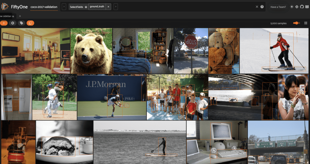
Now let’s generate detection predictions for these images from the command line as in the example above. For later convenience, we use this more general export_yolo_data() method.
def export_yolo_data(
    samples,
    export_dir,
    classes,
    label_field = "ground_truth",
    split = None
    ):

    if type(split) == list:
        splits = split
        for split in splits:
            export_yolo_data(
                samples,
                export_dir,
                classes,
                label_field,
                split
            )
    else:
        if split is None:
            split_view = samples
            split = "val"
        else:
            split_view = samples.match_tags(split)

        split_view.export(
            export_dir=export_dir,
            dataset_type=fo.types.YOLOv5Dataset,
            label_field=label_field,
            classes=classes,
            split=split
        )
For this data, the export and inference commands look like:
coco_val_dir = "coco_val"
export_yolo_data(dataset, coco_val_dir, coco_classes)
And:
yolo task=detect mode=predict model=yolov8n.pt source=coco_val/images/val save_txt=True save_conf=True
Now it’s time to add YOLOv8’s predictions for these images into our dataset. When we run a YOLOv8 inference task from the command line, the predictions are stored in a .txt file. For detections, these text files contain one line per object detection in the image: an integer for the class label, a class confidence score, and four values representing the bounding box.
We can read a YOLOv8 detection prediction file with N detections into an (N, 6) numpy array:
def read_yolo_detections_file(filepath):
    detections = []
    if not os.path.exists(filepath):
        return np.array([])

    with open(filepath) as f:
        lines = [line.rstrip('\n').split(' ') for line in f]

    for line in lines:
        detection = [float(l) for l in line]
        detections.append(detection)
    return np.array(detections)
From here, we need to convert these detections into FiftyOne’s Detections format.
YOLOv8 represents bounding boxes in a centered format with coordinates [center_x, center_y, width, height], whereas FiftyOne stores bounding boxes in [top-left-x, top-left-y, width, height] format. We can make this conversion by “un-centering” the predicted bounding boxes:
def _uncenter_boxes(boxes):
    '''convert from center coords to corner coords'''
    boxes[:, 0] -= boxes[:, 2]/2.
    boxes[:, 1] -= boxes[:, 3]/2.
Additionally, we can convert a list of class predictions (indices) to a list of class labels (strings) by passing in the class list:
def _get_class_labels(predicted_classes, class_list):
    labels = (predicted_classes).astype(int)
    labels = [class_list[l] for l in labels]
    return labels
Given the output of a read_yolo_detections_file() call, yolo_detections, we can generate the FiftyOne Detections object that captures this data:
def convert_yolo_detections_to_fiftyone(
    yolo_detections,
    class_list
    ):

    detections = []
    if yolo_detections.size == 0:
        return fo.Detections(detections=detections)

    boxes = yolo_detections[:, 1:-1]
    _uncenter_boxes(boxes)

    confs = yolo_detections[:, -1]
    labels = _get_class_labels(yolo_detections[:, 0], class_list)

    for label, conf, box in zip(labels, confs, boxes):
        detections.append(
            fo.Detection(
                label=label,
                bounding_box=box.tolist(),
                confidence=conf
            )
        )
    return fo.Detections(detections=detections)
The final ingredient is a function that takes in the file path of an image, and returns the file path of the corresponding YOLOv8 detection prediction text file.
def get_prediction_filepath(filepath, run_number = 1):
    run_num_string = ""
    if run_number != 1:
        run_num_string = str(run_number)
    filename = filepath.split("/")[-1].split(".")[0]
    return "runs/detect/predict{}/labels/".format(run_num_string) + filename + ".txt"
Note that if you run multiple inference calls for the same task, the predictions results are stored in a directory with the next available integer appended to predict in the file path. You can account for this in the above function by passing in the run_number argument.
Putting the pieces together, we can write a function that adds these YOLOv8 detections to all of the samples in our dataset efficiently by batching the read and write operations to the underlying MongoDB database.
def add_yolo_detections(
    samples,
    prediction_field,
    prediction_filepath,
    class_list
    ):

    prediction_filepaths = samples.values(prediction_filepath)
    yolo_detections = [read_yolo_detections_file(pf) for pf in prediction_filepaths]
    detections =  [convert_yolo_detections_to_fiftyone(yd, class_list) for yd in yolo_detections]
    samples.set_values(prediction_field, detections)
Now we can rapidly add the detections in a few lines of code:
filepaths = dataset.values("filepath")
prediction_filepaths = [get_prediction_filepath(fp) for fp in filepaths]
dataset.set_values(
    "yolov8n_det_filepath",
    prediction_filepaths
)

add_yolo_detections(
    dataset,
    "yolov8n",
    "yolov8n_det_filepath",
    coco_classes
)
Visualizing YOLOv8 predictions
The first step to understanding what a computer vision model is doing should also be to visualize the model’s predictions on your data. We can do so in the FiftyOne App:
session = fo.launch_app(dataset)
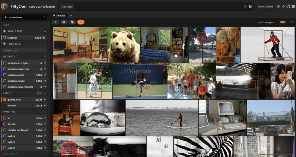
If we want to show only the predictions, we can uncheck the ground_truth label in the sidebar on the left. We can also view more details about the labels on an individual image by clicking on the image in the sample grid, which opens in an expanded modal.
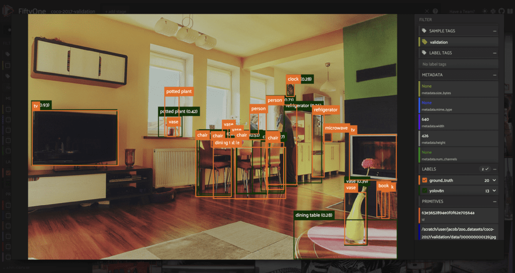
Here we can see the ground truth and predicted class labels, as well as the class confidence probabilities.
We can filter for high confidence predictions using the confidence slider in the sidebar on the left under the yolov8n label header:
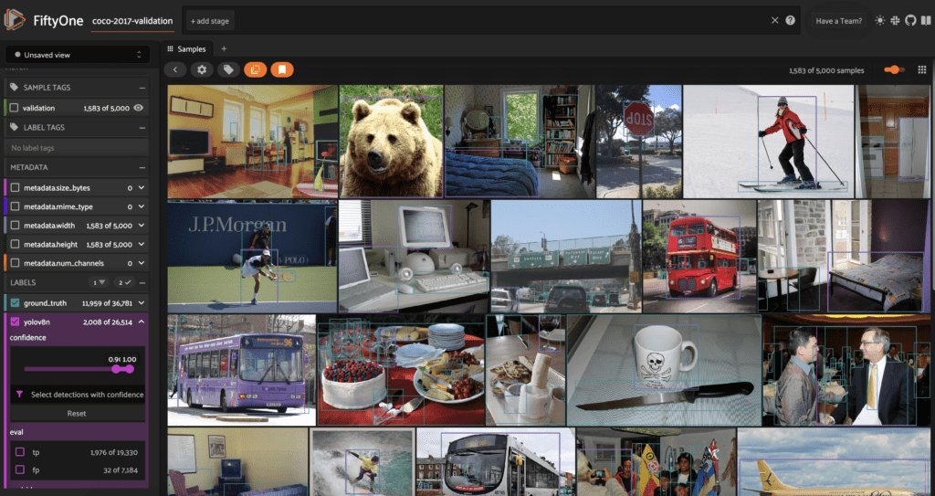
We can see that if we filter for predictions with confidence >= 0.9, we get only 2,008 out of the 26k+ predictions generated by running the model on the dataset.
It is also worth noting that it is possible to convert YOLOv8 predictions directly from the output of a YOLO model call in Python, without first generating external prediction files and reading them in. Let’s see how this can be done for instance segmentations.
Like detections, YOLOv8 stores instance segmentations with centered bounding boxes. In addition, YOLOv8 stores a mask that covers the entire image, with only a rectangular region of that mask containing nonzero values. FiftyOne, on the other hand, stores instance segmentations at Detection labels with a mask that only covers the given bounding box.
We can convert from YOLOv8 instance segmentations to FiftyOne instance segmentations with this convert_yolo_segmentations_to_fiftyone() function:
def convert_yolo_segmentations_to_fiftyone(
    yolo_segmentations,
    class_list
    ):

    detections = []
    boxes = yolo_segmentations.boxes.xywhn
    if not boxes.shape or yolo_segmentations.masks is None:
        return fo.Detections(detections=detections)

    _uncenter_boxes(boxes)
    masks = yolo_segmentations.masks.masks
    labels = _get_class_labels(yolo_segmentations.boxes.cls, class_list)

    for label, box, mask in zip(labels, boxes, masks):
        ## convert to absolute indices to index mask
        w, h = mask.shape
        tmp =  np.copy(box)
        tmp[2] += tmp[0]
        tmp[3] += tmp[1]
        tmp[0] *= h
        tmp[2] *= h
        tmp[1] *= w
        tmp[3] *= w
        tmp = [int(b) for b in tmp]
        y0, x0, y1, x1 = tmp
        sub_mask = mask[x0:x1, y0:y1]

        detections.append(
            fo.Detection(
                label=label,
                bounding_box = list(box),
                mask = sub_mask.astype(bool)
            )
        )
    return fo.Detections(detections=detections)
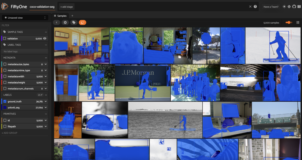
Looping through all samples in the dataset, we can add the predictions from our seg_model, and then view these predicted masks in the FiftyOne App.
Conclusion
In this article, we demonstrated how to start using YOLOv8 models on your data, and how to visualize YOLOv8 model predictions on images. In Part 2, using the same COCO validation images and labels, we’ll show you how to evaluate the quality of a YOLOv8 model’s predictions, identify edge cases, and assess potential modes of failure.
Continue to Part 2!
Join the FiftyOne community!
Join the thousands of engineers and data scientists already using FiftyOne to solve some of the most challenging problems in computer vision today!
- 1,350+ FiftyOne Slack members
- 2,500+ stars on GitHub
- 3,000+ Meetup members
- Used by 250+ repositories
- 55+ contributors

