Welcome to the latest installment of our ongoing blog series where we explore computer vision related datasets. In this post we’ll use the open source FiftyOne toolset to visualize Amazon’s recently released dataset for training “pick and place” robots, plus we’ll create embeddings with the OpenAI CLIP model to explore defects.
Wait, what’s FiftyOne?
FiftyOne is an open source computer vision toolset that enables data science teams to improve the performance of their computer vision models by helping them curate high quality datasets, evaluate models, find mistakes, visualize embeddings, and get to production faster.

What are “pick and place” robots?
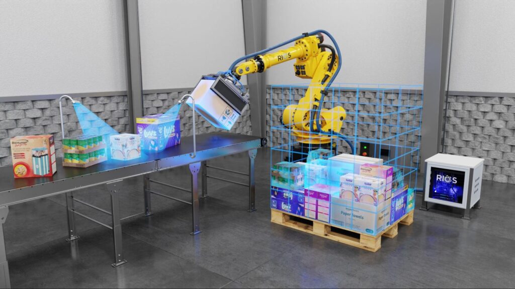
These days, pick and place robots are becoming more and more common in manufacturing and logistics environments. Leveraging robots that don’t require downtime (besides regularly scheduled maintenance) can boost overall production efficiency and free up humans to work on safer, less repetitive tasks. In some cases, humans and robots work side-by-side, leveraging the strengths of each.
Pick and place robots come in a variety of forms, with the most common type likely being the 5- or 6-axis articulated arm. There are also more specialized robots that can pick groups of items and place them in specific positions, robots designed to work at very high speeds, and the aforementioned collaborative robots or “cobots” that work in tandem with humans.
What are the practical applications of pick and place robots? Although manufacturing is the most obvious use case, you can also find these types of robots performing packaging, sorting, or inspection tasks that need to be done with speed and accuracy.
To learn more about the intersection between robots, manufacturing, and computer vision, check out: How Computer Vision Is Changing Manufacturing in 2023.
About the dataset
Earlier this month, Amazon publicly released the largest computer vision dataset ever captured in an industrial product-sorting setting. In contrast to previous datasets for robotic manipulation that might be limited either in the number of object types or in scene heterogeneity and realism, this new dataset, called ARMBench (Amazon Robotic Manipulation Benchmark), features more than 235,000 pick and place activities on 190,000 objects taking place in the context of an operating Amazon warehouse. This massive dataset can be used to train pick and place robots that are better able to generalize to new products and contexts.
To learn more about the motivations behind the dataset, check out the paper, ARMBench: An object-centric benchmark dataset for robotic manipulation over on the Amazon Science blog.
The basic scenario for ARMBench is one in which a robotic arm must retrieve a single item from a bin full of items and transfer it to a tray on a conveyor belt. According to the authors, “The variety of objects and their configurations and interactions in the context of the robotic system made for a uniquely challenging task.”
The ARMBench dataset is broken down as follows:
Defect detection
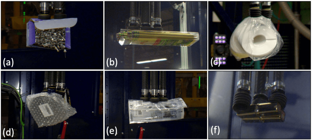
- Image defect detection (66 GB): This dataset comprises 13,303 images of objects with defects taken through multiple view-points (Transfer-images). For image defect detection, multi-pick and package-defects are the two defect classes. 100,000 images of objects with no defects or are available in the dataset. Multi-pick is used to describe activities where multiple objects were picked and transferred from the source container to the destination container. Package-defect is used to describe activities where the object packaging opened and/or the object separated into multiple parts. Two subclasses, open and deconstruction, are defined for package-defect.
- Video defect detection (255 GB): This dataset comprises 4,075 videos of objects with defects. Multi-picks are not as observable in videos and are excluded from this dataset. At the same time, open and deconstruction defects are observable in videos and are annotated. 100,000 videos of activities that did not result in a defect are available in the dataset.
Object identification
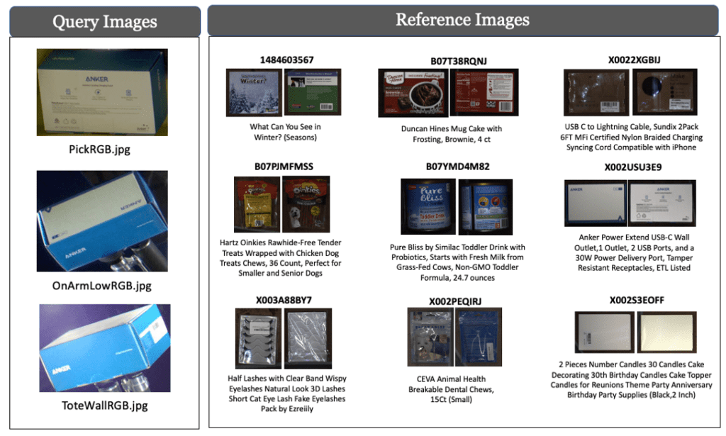
With Object identification the task is to identify an image segment as one of the objects within a database. In the pre-pick stage, identifying an object segment within the tote allows accessing any stored models or attributes of the object from past experience which can be used for manipulation planning purposes. In the post-pick stage, the ID has access to the segment of the object being manipulated both within the tote as well as when it is attached to the robotic arm.
- Picks: 235,000 pick activities with images of the picked object in tote and in robotic arm.
- Reference-images: Up to 6 images (1.jpg-6.jpg) corresponding to different product-ids.
Object segmentation
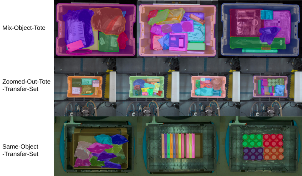
With this dataset, instance segmentation is used to identify and define distinct objects that are stored in containers. The outcomes of instance segmentation can be used to provide information to subsequent robotic processes, such as the identification of objects and generation of grasping strategies.
- Mix-Object-Tote (14 GB): This subset consists of close-up images of mixed objects that are stored in either yellow or blue totes. Mix-Object-Tote comprises a total of 44,253 images of size 2448 by 2048 pixels and 467,225 annotations, with an average of 10.5 instances per tote.
- Zoomed-Out-Tote-Transfer-Set (1.5 GB): This subset includes mixed objects placed in a yellow tote that were captured with sensors positioned further away from the tote, under different lighting conditions. The dataset contains 5,837 images of size 2046 by 2046 pixels and 43,401 annotations, with an average of 7.5 objects per tote.
- Same-Object-Transfer-Set (3 GB): This subset consists of multiple same objects placed in close proximity within various storage units. The Same-Object-Transfer-Set comprises 3,323 images of size 2048 by 1500 pixels and 12,664 annotations, with an average of 3.8 objects per scene.
Dataset quick facts
- Download: Request a download link from Amazon
- License: Creative Commons
- Paper: ARMBench: An object-centric benchmark dataset for robotic manipulation
- Authors: Chaitanya Mitash, Fan Wang, Shiyang Lu, Vikedo Terhuja, Tyler Garaas, Felipe Polido, Manikantan Nambi
Up next, let’s download the dataset, install FiftyOne, and import the dataset into the App so we can visualize it!
Step 1: Download the dataset
In order to load the ARMBench dataset into FiftyOne, you’ll need to request a download link from Amazon. For the purposes of this blog, we’ll be focusing on the Image Defect Detection subset of data that is part of the larger ARMBench dataset.
Step 2: Install FiftyOne
pip install fiftyone
If you don’t already have FiftyOne installed on your laptop, it takes less than a minute! Learn more about how to get up and running with FiftyOne in the Docs.
Step 3: Import the dataset
Now that you have the dataset downloaded and FiftyOne installed, let’s import the dataset, make it compatible with FiftyOne and launch the FiftyOne App.
from os import path
import glob
import json

import numpy as np
import imagesize

import fiftyone as fo

# set to download path
image_defect_root = '/PATH TO ARMBENCH DATASET GOES HERE'

# maximum number of groups to load (set to None for entire dataset)
max_groups = 100

data_root = path.join(image_defect_root,'data')
train_csv = path.join(image_defect_root,'train.csv')
test_csv = path.join(image_defect_root,'test.csv')


def readlines(f):
    with open(f,'r') as fh:
        lines = [line.strip() for line in fh]
    return lines


def load_json(f):
    with open(f,'r') as fh:
        j = json.load(fh)
    return j
To get started, we import FiftyOne and set up some paths and utility functions. The images and annotations live in subfolders under data_root.
The basic building block of a FiftyOne dataset is a sample – in this case, an image along with its annotations and metadata. This dataset has additional structure, as each data subfolder contains multiple images (typically, four) taken of a single object. This structure lends itself naturally to using a grouped dataset in FiftyOne. The max_groups parameter limits the number of groups (or subfolders) of data that are imported, as this is a large dataset.
def parse_data_dir(data_dir):
    """Parse one data directory (group)

    Args:
        data_dir: full path to a single data folder, eg <image_defect_root>/data/<id>

    Returns:
        id, <list of dict>
    """

    id = path.basename(data_dir)
    jpg_pat = path.join(data_dir,'*.jpg')
    ims = sorted(glob.glob(jpg_pat))
    jsons = [path.splitext(x)[0]+'.json' for x in ims]
    jsons = [load_json(x) for x in jsons]

    imsbase = [path.basename(x) for x in ims]
    imskey = [path.splitext(x)[0] for x in imsbase]
    json_files = [path.join(data_dir,x+'.json') for x in imskey]
    jsons = [load_json(x) for x in json_files]

    for im, json in zip(ims,jsons):
        imbase = path.basename(im)
        imkey = path.splitext(imbase)[0]
        assert json['id']==imbase or json['id']==imkey
        assert imkey.startswith(id + '_')
        slice = imkey[len(id)+1:]

        imw,imh = imagesize.get(im)
        new_info = {
            'filepath': im,
            'imw': imw,
            'imh': imh,
            'slice': slice,
        }
        json.update(new_info)

    return id, jsons


def parse_all_data_dirs():
    """Parse all data folders, up to max_groups

    Returns:
        list of (id,jsons)
    """

    data_dirs = sorted(glob.glob(path.join(data_root,'*')))
    data_dirs = data_dirs[:max_groups]
    data_dir_infos = [parse_data_dir(x) for x in data_dirs]
    return data_dir_infos
parse_data_dir parses a single subfolder of data. Each image has a corresponding json file that contains a segmentation polygon of the object, as well as labels indicating whether the transfer was without defect, or if a defect occurred, the type and subtype of defect observed.
We augment the dictionaries read from the annotation files with image metadata and a slice identifier, which just specifies the camera view (1-4) for that image.
The image height and width will be important because the annotation polygons in this dataset are stored as absolute pixel values, whereas FiftyOne stores vertices normalized to image dimensions. We will perform the conversion when we create our samples.
Let’s create our FiftyOne dataset!
train_set = set(readlines(train_csv))
test_set = set(readlines(test_csv))
data_dir_infos = parse_all_data_dirs()

dataset = fo.Dataset('ARMBench-Image-Defect-Detection')
dataset.persistent = True

samples_all = []

for id, grp_info in data_dir_infos:

    group = fo.Group()

    for info in grp_info:
        if id in train_set:
            tags = ['train']
        elif id in test_set:
            tags = ['test']
        else:
            tags = []

        if info['label']:
            tags.append(info['label'])
        if info['sublabel']:
            tags.append(info['sublabel'])

        sample = fo.Sample(filepath=info['filepath'],
                           tags=tags,
                           group=group.element(info['slice']))

        imw = info['imw']
        imh = info['imh']
        poly_pts = info['polygon']
        if poly_pts:
            poly_pts = np.array(poly_pts,dtype=np.float64)
            poly_pts[:,0] /= imw
            poly_pts[:,1] /= imh
            polyline = fo.Polyline(points=[poly_pts.tolist()],filled=True)
            detections = fo.Polylines(polylines=[polyline]).to_detections(frame_size=(imw,imh))
            sample['object'] = detections

        samples_all.append(sample)

dataset.add_samples(samples_all)
The basic recipe for loading a dataset into FiftyOne is simple: create a Dataset, then create and add Samples! Here we have groups as well, and we follow this basic recipe for adding samples to a grouped dataset.
We’ll use FiftyOne tags to store our defect annotations, as well as membership in train and test splits. This makes it a snap to visualize and filter by these elements in the App.
We have a couple options for our object polygons. We could represent these in FiftyOne as either polylines or instance segmentations. The bounding box will come in handy later, so we use instance segmentations in the end. But to get there, we first load into a Polyline and then do a conversion, as Polylines easily accept the list-of-vertices format of these annotations. FiftyOne has support for a huge variety of label types and dataset formats, making it a snap to work with all types of data in the way that works best for you.
Step 4: Launch the FiftyOne App to visualize the dataset
session = fo.launch_app(dataset)
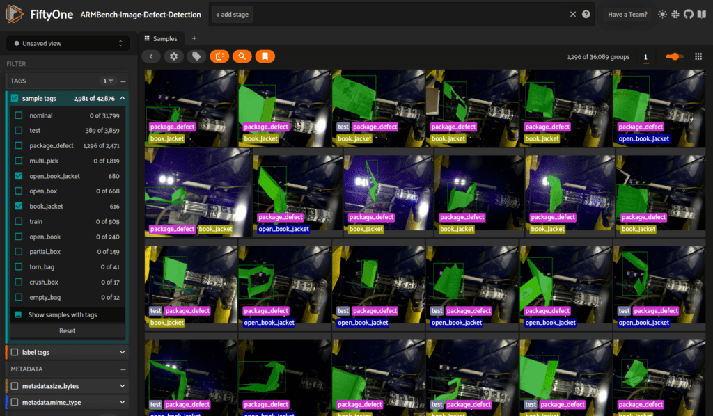
With our dataset created, let’s launch the FiftyOne App in a browser. You should see the following initial view of the ARMBench-Image-Defect-Detection dataset by default in the App:

Tags
We’ve loaded our annotations as FiftyOne tags. In the sidebar, click on Tags > sample tags to have these tags populate the samples in the App. By selecting certain tags, you can restrict your view to show (for instance) only those tags of interest. Here, we are focusing on open book jackets.
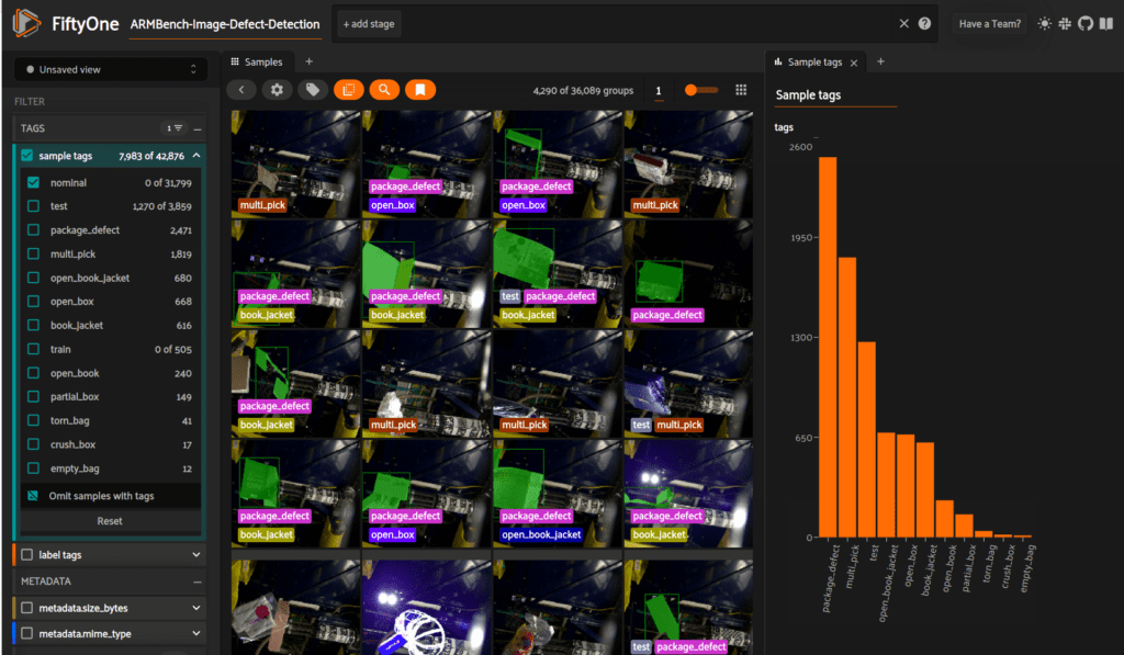
Histograms
We can explore the distribution of tags or annotations using FiftyOne’s histogram panel. In this view, we’ve excluded nominal samples and are focusing on defects. The histogram shows us a breakdown of the distribution of the various defect annotations.
Note that the defect tags are not mutually exclusive. As the paper describes, the defects in this dataset fall into two overall categories: package_defect and multi_pick. Some of the tags then further detail the type of defect within these categories. Open book jackets are relatively common, while crushed boxes (fortunately for customers!) are less so.
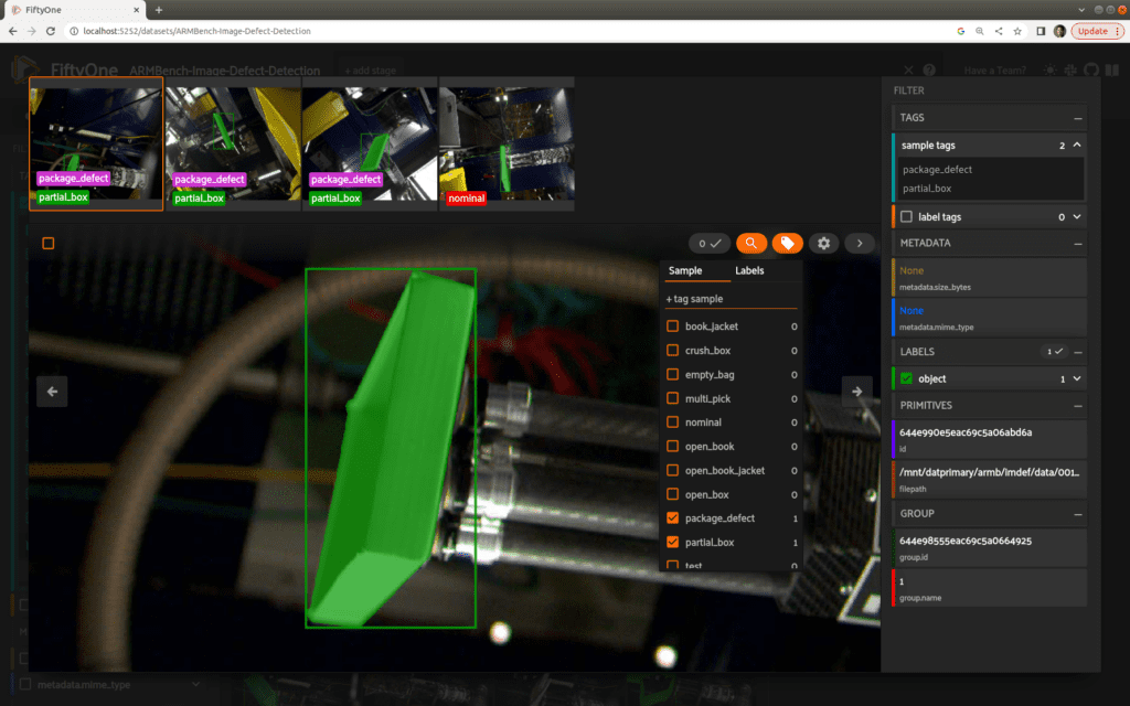
Sample details
Click on any of the samples to get a larger view with additional view tools and details available. In this image, we’ve used the crop tool to zoom tightly around the object of interest.
The image carousel at the top of the interface shows the other views or slices for this sample. Any of these images may be selected to become the primary displayed image. Note that while the first three slices show the same defect tags, the fourth view is listed as nominal. The partial box defect is only visible from certain angles, making multi-view grouped datasets like this one crucial in this type of application.
Embeddings and the FiftyOne Brain
By browsing our data in the FiftyOne App, we can get a pretty good sense of what our data looks like, including how the various defects manifest and how camera views differ from each other.
This is just the beginning. Let’s dig into our data deeper with the FiftyOne Brain and its embeddings functionality. If you are new to embeddings, check out this post over on the Towards Data Science blog.
The ARMBench dataset comes with tasks or challenges associated with each data subset. In our case, the task at hand is defect detection. This is a difficult problem, as defects are often rare and unpredictable in nature, challenging supervised learning approaches. The difficulty is magnified here given the huge variety of objects and packaging present. Can analyzing embeddings in FiftyOne help shed some light on the challenge of finding and identifying pick and place defects?
To start things off, we’ll import the FiftyOne Brain. We’ll focus on the fourth slice of our data, which from our exploration in FiftyOne seems qualitatively less noisy in background and lighting heterogeneity. Our analysis will compute embeddings on detection patches, so we’ll also filter out the relatively small number of samples that do not have object detections. (This includes the multi-pick defects, as these do not have accompanying segmentations.) For simplicity, we clone a new, smaller dataset restricted to this slice of samples.
import fiftyone.brain as fob
from fiftyone import ViewField as F
dataset = dataset.select_group_slices('4') \
                 .filter_labels('object',F()) \
                 .clone(name='ArmBench-Image-Defect-Slice4',persistent=True)
To assist in visualizing our embeddings, we’ll assign a label field to our object detections based on our tags. In addition to the nominal label, there are two basic types of defects, multi-pick and package-defect. Package-defects are broken down further for books, boxes, and bags. To simplify the visualizations, we’ll collapse the book-related and bag-related defects into single categories.
labels = {
    'book': ['book_jacket','open_book_jacket','open_book'],
    'open_box': ['open_box'],
    'partial_box':['partial_box'],
    'crush_box':['crush_box'],
    'bag': ['empty_bag','torn_bag'],
    'multi_pick': ['multi_pick'],
    'nominal': ['nominal'],
}

# set default defect label; this is overwritten for most samples
dataset.set_values('object.detections.label',[['other_defect']]*len(dataset))

for ty,tags in labels.items():
    view = dataset.match_tags(tags)
    view.set_values('object.detections.label',[[ty]]*len(view))
It’s time to compute our embeddings! We’ll use the OpenAI CLIP model from the FiftyOne Model Zoo to compute embeddings on our object patches. Meanwhile, the FiftyOne Brain compute_visualization method will use the UMAP method to perform structure-preserving dimensionality reduction to enable a 2D visualization.
fob.compute_visualization(dataset,
                          patches_field='object',
                          embeddings='clip_embeddings',
                          brain_key='object_clip',
                          model='clip-vit-base32-torch')
In this method call:
patches_fieldspecifies that we will compute embeddings on the bounding box patches (or crops) for the detections stored in theobjectfield.embeddingsnames a field to store our computed embedding vectors. For the CLIP model, these are 512-dimensional vectors.brain_keygives an identifier to this visualization, so we can refer to it later and in the FiftyOne App.modelspecifies a model from the FiftyOne Model Zoo. The pixels from our detection crops are passed through this model to generate our embedding vectors.
In the FiftyOne App, we’ll enter a Patches view to focus on our detected objects and their corresponding embeddings. Using the FiftyOne Embeddings panel, it’s easy to visualize these patch embeddings, colored by label type:
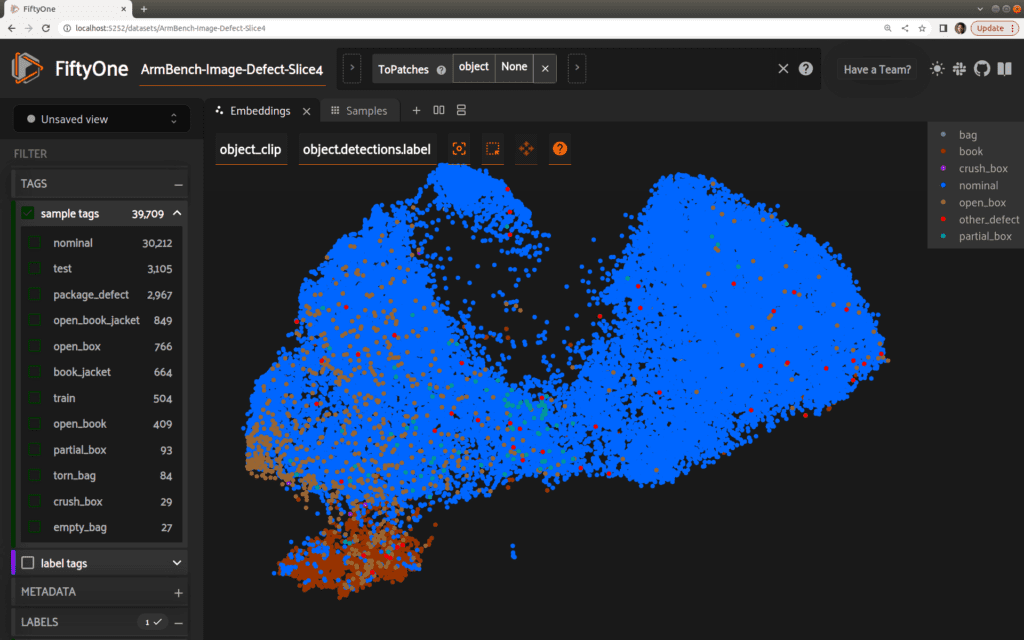
As it turns out, our book defects are clustered quite visibly in the lower-left-hand corner! Using the lasso tool, we can select this group of samples. In the samples grid, it is clear that the majority of these samples are indeed defects, and in particular, book defects:
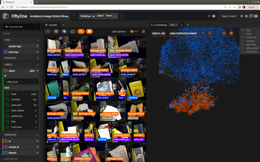
Setting rigor aside for a moment, this lasso-ed selection of 1830 objects captures 1560 book-related defects out of a total of 1922 in the entire dataset, for a recall of 1560/1922 ~ 81%. The remaining 270 selected samples represent false positives in a pool of 31257 negatives, for a false positive rate of 270/31257 ~ .8%. (Recall and false positive rate are the preferred metrics described in the paper). Of course, this is only a rough exploration, but it is suggestive of the rich structure and information available in these embeddings.
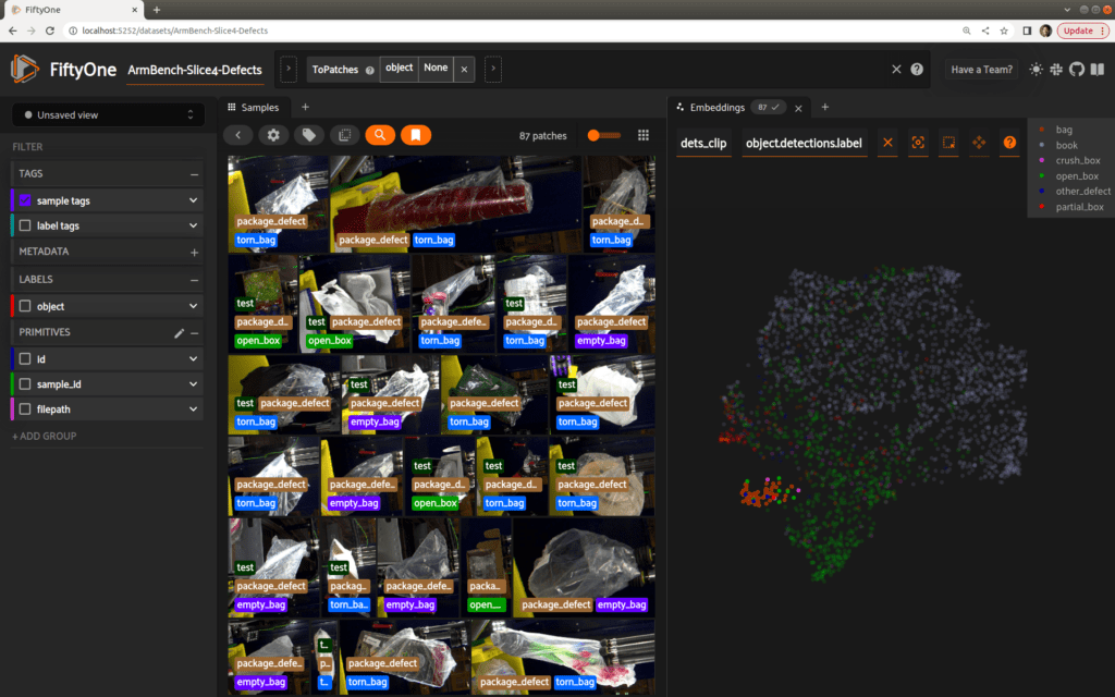
What if we just focus on samples with defects? We’ll re-use our computed embeddings, but re-compute the visualization against the smaller subset of data:
view_defects = dataset.match_tags('nominal',bool=False)

fob.compute_visualization(view_defects,
                          patches_field='object',
                          embeddings='clip_embeddings',
                          brain_key='dets_clip')

session = fo.launch_app(view_defects)
Again, some clear structure is evident in our embeddings plot. Bag-related defects, for instance, are clustered quite tightly, as selected and shown here.
Pretty cool stuff! It’s not the end of the story, but this analysis has definitely generated some insights for us and kick-started our effort on detecting defects in this novel dataset.
Let’s take a step back and return to our first embeddings plot, which includes all samples from slice 4. While we have detailed labels for defects, the large mass of nominal samples lacks annotations. You may have noticed however that the embeddings plot already gives some clues about structure in this sea of data. Selecting a cluster near the top of the mass, for instance, reveals a distinct clustering of plastic bottles!
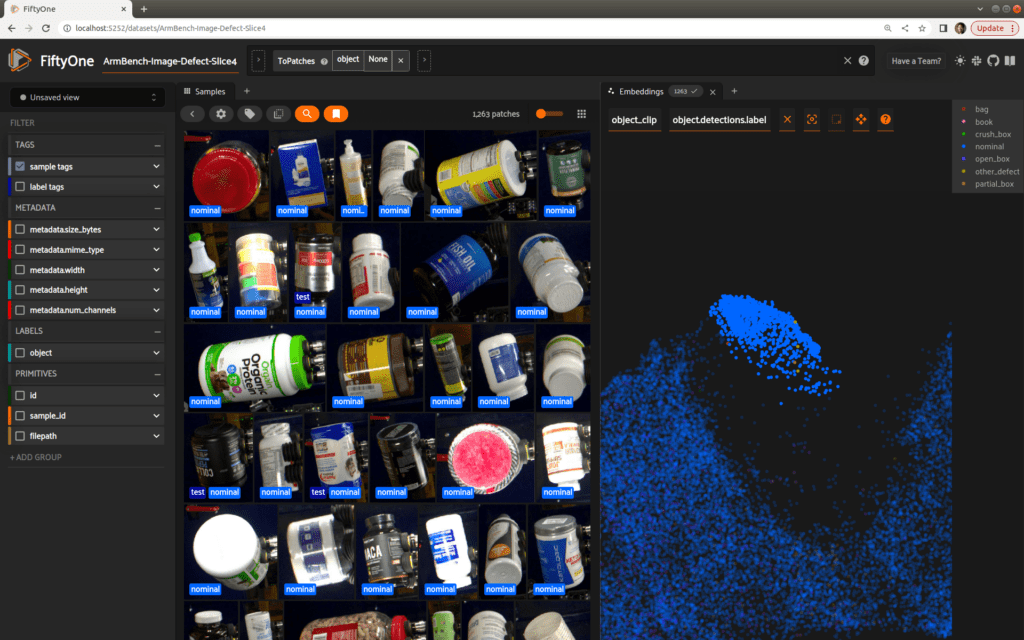
The other ‘lobes’ of the visualization are semantically meaningful as well, representing distinct clusters of cardboard boxes and objects wrapped in plastic.
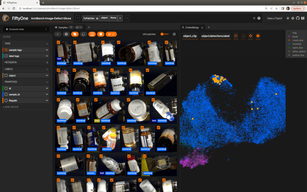
As a final example of the tools available in the FiftyOne Brain, let’s utilize the natural language capabilities of our CLIP embeddings to search by the text prompt “medicine bottle”, returning the top 100 matches. The returned results are quite consistent, and overwhelmingly located in the cluster of bottles we found earlier. Depending on our analysis, we could leverage this zero-shot labeling capability to automatically add annotations to our dataset to give us more to work with in the large sea of nominal samples.
You can see more in this short video.
Start working with the dataset
That’s a wrap for now! We hope you enjoyed this quick exploration of defect detection and the new ARMBench dataset. We’ll be adding this massive dataset to the FiftyOne Dataset Zoo in the near future, so you’ll be able to explore it on your own in just a couple lines of Python!

