Yesterday, Deci AI released a new state of the art object detection model named YOLO-NAS, which achieves higher mean average precision than prior models running with the same latency.
In this blog post, we’ll show you how to generate predictions with YOLO-NAS and load them into FiftyOne! If you are new to FiftyOne, it is an open source computer vision toolset for curating better data and building better models.
Setup
If you haven’t done so already, you will need to install FiftyOne:
pip install fiftyone
You will also need to install Deci AI’s SuperGradients package:
pip install super-gradients
The next step is importing FiftyOne and loading a dataset from the FiftyOne Dataset Zoo. We will use a random subset of the validation split from the MS COCO dataset. We will also make the dataset persistent:
import fiftyone as fo
import fiftyone.zoo as foz
dataset = foz.load_zoo_dataset(
"coco-2017",
split = "validation",
max_samples=1000
)
dataset.name = "YOLO-NAS-demo"
dataset.persistent = True
We will also use the compute_metadata() method to store image width and height, so that we can use these to convert between absolute and relative coordinates for bounding boxes:
dataset.compute_metadata()
Now we load in the YOLO-NAS model. We’ll use the large architecture (hence the “l”) and will download pretrained weights for a version of the model trained on COCO data. For a list of available weights, see here.
from super_gradients.training import models
model = models.get("yolo_nas_l", pretrained_weights="coco")
Generating YOLO-NAS Predictions
We can generate predictions for a single sample by passing the filepath for the sample’s image to our model’s `predict()` method, along with an optional confidence threshold:
sample = dataset.first()
prediction = model.predict(sample.filepath, conf = 0.25)
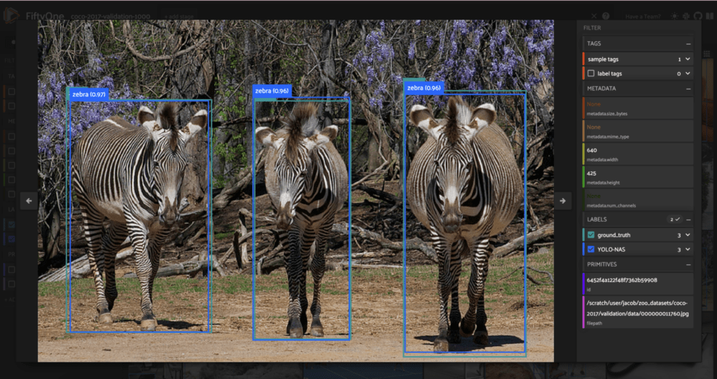
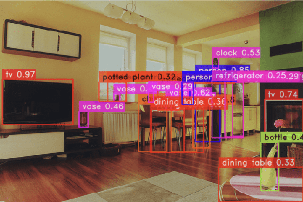
We can then visualize the object bounding boxes drawn onto the image with the show() method for the SuperGradient DetectionResult:
prediction.show()
To efficiently generate predictions for all of the images in our dataset, we batch these operations by passing the model the names of all the filepaths for all of our images:
fps, widths, heights = dataset.values(
        ["filepath", "metadata.width", "metadata.height"]
    )

    ## batch predictions
    preds = model.predict(fps, conf = confidence)._images_prediction_lst
To load these predictions into FiftyOne, we need to first convert these into Detection label objects. This will require accessing the internals of the prediction objects, extracting the confidence, labels, and bounding boxes.
We can access this information via the _images_prediction_lst attribute of the prediction objects. Let’s see what this looks like for a single image.
pred = model.predict(sample.filepath, conf = 0.9)
print(next(pred._images_prediction_lst))
ImageDetectionPrediction(image=array([[[170, 136,  73],
        [173, 142,  77],
        [175, 144,  79],
        ...,
        [ 69,  76,  42],
        [ 68,  76,  39],
        [ 70,  71,  37]],

       [[172, 141,  77],
        [176, 145,  80],
        [177, 146,  81],
        ...,
        [ 69,  77,  40],
        [ 72,  80,  43],
        [ 71,  75,  40]],

       [[175, 144,  79],
        [177, 146,  81],
        [178, 147,  80],
        ...,
        [ 70,  78,  39],
        [ 69,  77,  40],
        [ 71,  75,  40]],

       ...,

       [[188, 189, 157],
        [183, 183, 149],
        [193, 187, 153],
        ...,
        [186, 157, 153],
        [186, 157, 153],
        [187, 156, 154]],

       [[186, 183, 152],
        [187, 184, 153],
        [186, 183, 152],
        ...,
        [198, 134, 134],
        [195, 120, 124],
        [186,  88, 101]],

       [[186, 183, 150],
        [187, 184, 151],
        [186, 183, 152],
        ...,
        [129,  60,  63],
        [126,  57,  60],
        [107,  41,  45]]], dtype=uint8), prediction=DetectionPrediction(bboxes_xyxy=array([[  5.661982, 166.75662 , 154.55098 , 261.8113  ],
       [292.11624 , 217.75893 , 352.51135 , 318.72244 ]], dtype=float32), confidence=array([0.96724653, 0.9323513 ], dtype=float32), labels=array([62., 56.], dtype=float32)), class_names=['person', 'bicycle', 'car', 'motorcycle', 'airplane', 'bus', 'train', 'truck', 'boat', 'traffic light', 'fire hydrant', 'stop sign', 'parking meter', 'bench', 'bird', 'cat', 'dog', 'horse', 'sheep', 'cow', 'elephant', 'bear', 'zebra', 'giraffe', 'backpack', 'umbrella', 'handbag', 'tie', 'suitcase', 'frisbee', 'skis', 'snowboard', 'sports ball', 'kite', 'baseball bat', 'baseball glove', 'skateboard', 'surfboard', 'tennis racket', 'bottle', 'wine glass', 'cup', 'fork', 'knife', 'spoon', 'bowl', 'banana', 'apple', 'sandwich', 'orange', 'broccoli', 'carrot', 'hot dog', 'pizza', 'donut', 'cake', 'chair', 'couch', 'potted plant', 'bed', 'dining table', 'toilet', 'tv', 'laptop', 'mouse', 'remote', 'keyboard', 'cell phone', 'microwave', 'oven', 'toaster', 'sink', 'refrigerator', 'book', 'clock', 'vase', 'scissors', 'teddy bear', 'hair drier', 'toothbrush'])
Because the _images_prediction_lst attribute is a generator, we used next() to see what it generates, which is an ImageDetectionPrediction object. In this result, we can see bounding boxes stored in xyxy format, an array of confidence scores, and an array of integers representing the indices of the label classes in the class_names array for those detections. The class names are precisely the COCO class names.
Here is how we can convert bounding boxes from YOLO-NAS output coordinates:
def convert_bboxes(bboxes, w, h):
    tmp = np.copy(bboxes[:, 1])
    bboxes[:, 1] = h - bboxes[:, 3]
    bboxes[:, 3] = h - tmp
    bboxes[:, 0]/= w
    bboxes[:, 2]/= w
    bboxes[:, 1]/= h
    bboxes[:, 3]/= h
    bboxes[:, 2] -= bboxes[:, 0]
    bboxes[:, 3] -= bboxes[:, 1]
    bboxes[:, 1] = 1 - (bboxes[:, 1] + bboxes[:, 3])
    return bboxes
Applying this bounding box conversion, we can generate FiftyOne Detection objects for each object, and create a Detections object containing a list of detected objects for a given image:
def generate_detections(p, width, height):
    class_names = p.class_names
    dp = p.prediction
    bboxes, confs, labels = np.array(dp.bboxes_xyxy), dp.confidence, dp.labels.astype(int)
    if 0 in bboxes.shape:
        return fo.Detections(detections = [])

    bboxes = convert_bboxes(bboxes, width, height)
    labels = [class_names[l] for l in labels]

    detections = [
        fo.Detection(
            label = l,
            confidence = c,
            bounding_box = b
        )
        for (l, c, b) in zip(labels, confs, bboxes)
    ]
    return fo.Detections(detections=detections)
Putting it all together, we can efficiently add YOLO-NAS detection predictions to our dataset:
def add_YOLO_NAS_predictions(dataset, confidence = 0.9):
    ## aggregation to minimize expensive operations
    fps, widths, heights = dataset.values(
        ["filepath", "metadata.width", "metadata.height"]
    )

    ## batch predictions
    preds = model.predict(fps, conf = confidence)._images_prediction_lst

    ## add all predictions to dataset at once
    dets = [
        generate_detections(pred, w, h)
        for pred, w, h in zip(preds, widths, heights)
    ]
    dataset.set_values("YOLO-NAS", dets)
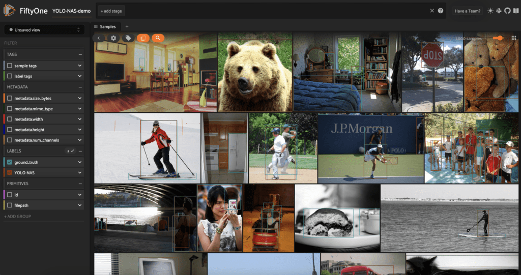
Applying this to our dataset and launching a session of the FiftyOne App, we can visualize the results:
add_YOLO_NAS_predictions(dataset, confidence = 0.7)
session = fo.launch_app(dataset)
Evaluation
With the data loaded into FiftyOne, we can evaluate the quality of the object detection predictions against the “ground truth” with FiftyOne’s evaluate_detections() method. We will store the results with an evaluation key so we can view the resulting evaluation patches in the FiftyOne App:
res = dataset.evaluate_detections(
    "YOLO-NAS",
    eval_key="eval_yolonas"
)
session.view = dataset.to_evaluation_patches("eval_yolonas")
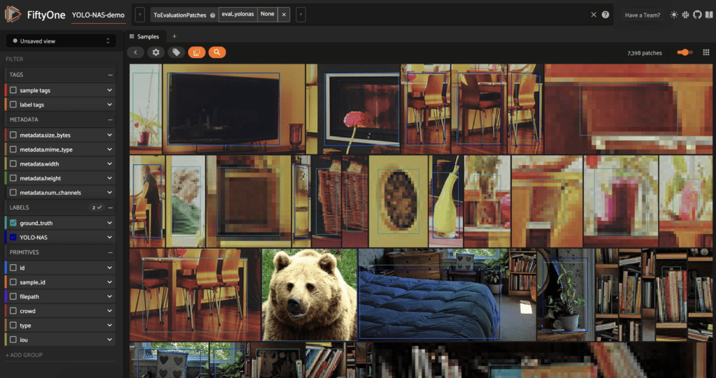
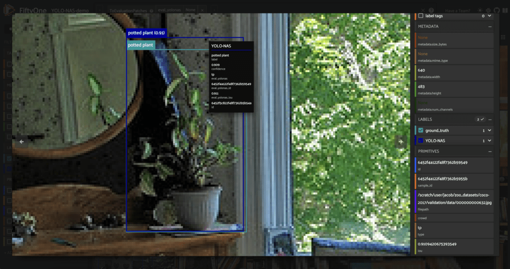
We can click into one of these evaluation patches and, hovering over the detection, we can see attributes like intersection over union (IoU) score, and whether the prediction was a true positive, false positive, or false negative.
If we wanted to see images with the most false positives, we could sort the dataset accordingly:
### get images with the most FP's first
fp_view = dataset.sort_by("eval_yolonas_fp", reverse = True)
We can also dig into the performance data more quantitatively by printing metrics for the most commonly occurring classes in the dataset:
counts = dataset.count_values("ground_truth.detections.label")
classes_top10 = sorted(counts, key=counts.get, reverse=True)[:10]
# Print a report for the top-10 classes
res.print_report(classes=classes_top10)
              precision    recall  f1-score   support

      person       0.98      0.52      0.68      2259
       chair       0.88      0.33      0.48       401
         car       0.93      0.42      0.58       348
        book       1.00      0.03      0.06       212
      bottle       0.88      0.28      0.43       210
         cup       0.97      0.45      0.61       185
dining table       0.85      0.18      0.30       153
        bowl       0.86      0.34      0.49       128
        bird       1.00      0.39      0.56       103
    backpack       1.00      0.07      0.13        98

   micro avg       0.95      0.42      0.58      4097
   macro avg       0.93      0.30      0.43      4097
weighted avg       0.95      0.42      0.57      4097
Conclusion
If you want to take this further, you may be interested in:
- Applying YOLO-NAS to video data, and loading these predictions into FiftyOne
- Fine-tuning YOLO-NAS on your own data, and using FiftyOne’s Evaluation API to compare the base and fine-tuned models
Join the FiftyOne community!
Join the thousands of engineers and data scientists already using FiftyOne to solve some of the most challenging problems in computer vision today!
- 1,500+ FiftyOne Slack members
- 2,900+ stars on GitHub
- 3,900+ Meetup members
- Used by 266+ repositories
- 58+ contributors

