FACET: A Benchmark Dataset for Fairness in Computer Vision

Everything you need to know!

Computer vision has come a long way over the past few years. Between single-stage detectors, neural architecture search, vision transformers, and foundation models, challenges that once seemed insurmountable are now standard fare. There are even high quality zero-shot models for detection (such as Grounding DINO) and segmentation (SAM, FastSAM), so for many applications, you can achieve a good baseline without any custom training!

As computer vision models have rapidly improved, the problem of bias has increasingly reared its head and become increasingly pronounced: even models that achieve state-of-the-art performance on one-number metrics like mean average precision or F1 score can vary wildly in their ability to generate predictions for people of different demographics, genders, and skin tones. If you’re curious to learn more about how models can learn human biases, check out this paper (cited by the FACET team).

In an effort to address these biases, a team at Meta has released FACET (FAirness in Computer Vision EvaluaTion), a new benchmark dataset for studying and evaluating the “fairness” in computer vision models. When developing FACET, the team set out to create the most comprehensive, diverse fairness benchmark dataset to date.

This blog will give you everything you need to know to get started working with FACET so you can ensure that the models you deploy are not learning biases.

• FACET Dataset Quick Facts
• Loading Ground Truth Annotations
• Evaluating Bias in Your Models

FACET Dataset Quick Facts

Paper

• Title: FACET: Fairness in Computer Vision Evaluation Benchmark — ICCV 2023
• Authors: Laura Gustafson, Chloe Rolland, Nikhila Ravi, Quentin Duval, Aaron Adcock, Cheng-Yang Fu, Melissa Hall, Candace Ross | Meta AI

Dataset

• License
• Data Card
• ⚠️Only to be used for evaluation purposes, NOT for training purposes

Annotations

• annotations/annotations.csv: person detections with bounding boxes and attributes (see data card for details)
• annotations/coco_boxes.json: MS COCO formatted detection bounding boxes for people, without attributes
• annotations/coco_masks.json: MS COCO formatted segmentation masks for people, clothing, and hair — encoded with Run-Length Encoding (RLE) — and bounding boxes

Dataset Statistics

• 31,702 images (a subset of the SA-1B dataset)
• 49,551 unique person detections, spanning protected attributes, unprotected attributes, lighting conditions, and more.
• 69,105 instance segmentation masks (person, clothing, and hair)
• 52 person-related classes (all person detections have a primary; some also have a secondary class)
• Perceived skin tone label interpretation: 1–10 on Monk Skin Tone scale

Efforts Taken by FACET Team to Ensure Fairness

• Expert annotators: the team hired experts from multiple geographic regions, from the Americas to Southeast Asia. Annotators also completed “stage-specific training” before they could begin labeling.
• Perceived labels: protected attributes (age, gender presentation, and skin tone) are labeled as “perceived” to reflect the limitations of image annotation. For instance for age, the team writes: “it is impossible to tell a person’s true age from an image, these numerical ranges are a rough guideline to delineate each perceived age group”.
• Diverse scenarios: from different lighting conditions and degrees of occlusion, to varied numbers of people in the image and an array of accessories, the FACET team tried to capture a broad range of visual scenarios. In addition to evaluating how model performance depends on a single demographic variable, this allows for evaluations of intersectionality.
• Image filtering: to avoid inheriting biases from existing detection and classification models, the FACET team employed human annotators to filter out images that did not contain a person matching one of the 52 label categories (singer, painter, astronaut, …). This filtered out about 80% of the initial images.
• Class disambiguation: sometimes a person fits the description of more than one label class. As the FACET authors illustrate, “a person playing the guitar and singing can match the category labels guitarist and singer”. To account for this, a secondary class label is given to detected persons when appropriate.
• Skin tone aggregation: because the tone of one’s skin can influence how they perceive others’ skin tones, FACET aggregates perceived skin tone values across multiple annotators for each label.

Value Counts by Attribute

• Lighting Condition

well lit: 35533
underexposed: 1313
overexposed: 553
dimly lit: 10955
None/na: 1197

• Hair Type

straight: 18382
curly: 719
bald: 1017
wavy: 6141
dreadlocks: 280
coily: 458
None/na: 22554

• Hair Color

black: 14041
blonde: 2249
red: 333
colored: 248
brown: 10668
grey: 2107
None/na: 19905

• Has Facial Hair

True: 6121
False: 43430

• Perceived Age Presentation

young (25-40): 8860
middle (41-65): 27380
older (65+): 2659
None: 10652

• Perceived Gender Presentation

fem: 10245
masc: 33240
non binary: 95
None/na: 5971

• Tattoo

False: 48846
True: 705

Primary Class (in alphabetical order)

astronaut': 286,
'backpacker': 1612,
'ballplayer': 1309,
'bartender': 56,
'basketball_player': 1668,
'boatman': 2048,
'carpenter': 223,
'cheerleader': 399,
'climber': 455,
'computer_user': 1164,
'craftsman': 1034,
'dancer': 1397,
'disk_jockey': 310,
'doctor': 802,
'drummer': 977,
'electrician': 468,
'farmer': 1542,
'fireman': 913,
'flutist': 302,
'gardener': 457,
'guard': 1361,
'guitarist': 1180,
'gymnast': 615,
'hairdresser': 458,
'horseman': 735,
'judge': 96,
'laborer': 2540,
'lawman': 4455,
'lifeguard': 511,
'machinist': 354,
'motorcyclist': 1367,
'nurse': 1042,
'painter': 898,
'patient': 884,
'prayer': 798,
'referee': 755,
'repairman': 1295,
'reporter': 470,
'retailer': 546,
'runner': 638,
'sculptor': 213,
'seller': 1178,
'singer': 1286,
'skateboarder': 990,
'soccer_player': 1226,
'soldier': 1457,
'speaker': 1416,
'student': 682,
'teacher': 192,
'tennis_player': 1661,
'trumpeter': 498,
'waiter': 332

Loading the FACET Dataset

Prerequisites

Before you download the dataset, you need to sign Meta’s FACET usage agreement here. After doing so, unzip the four zip files (annotations, imgs_1, imgs_2, and imgs_3).

We will be using the open source computer vision library FiftyOne for data management and visualization, so if you have not done so already, install FiftyOne:

pip install fiftyone

In Python, import the needed libraries:

import json
import numpy as np
import os
import pandas as pd
from PIL import Image
from pycocotools import mask as maskUtils
from tqdm.notebook import tqdm

As well as the FiftyOne modules we will be utilizing:

import fiftyone as fo
import fiftyone.brain as fob
import fiftyone.zoo as foz
from fiftyone import ViewField as F

Creating the Dataset

Now we are ready to create the dataset. We will create an empty dataset (and persist it to database), and then add all of the images in each of the three image folders we unzipped:

## use relative paths to your image dirs
IMG_DIRS = ["imgs_1", "imgs_2", "imgs_3"]

dataset = fo.Dataset(name = "FACET", persistent=True)

for img_dir in IMG_DIRS:
dataset.add_images_dir(img_dir)

dataset.compute_metadata()

We also compute the “metadata” so that we can utilize sample width and height when converting between relative and absolute bounding box conventions.

We can print out the dataset and get some quick facts:

print(dataset)

Name: FACET
Media type: image
Num samples: 31702
Persistent: True
Tags: []
Sample fields:
id: fiftyone.core.fields.ObjectIdField
filepath: fiftyone.core.fields.StringField
tags: fiftyone.core.fields.ListField(fiftyone.core.fields.StringField)
metadata: fiftyone.core.fields.EmbeddedDocumentField(fiftyone.core.metadata.ImageMetadata)

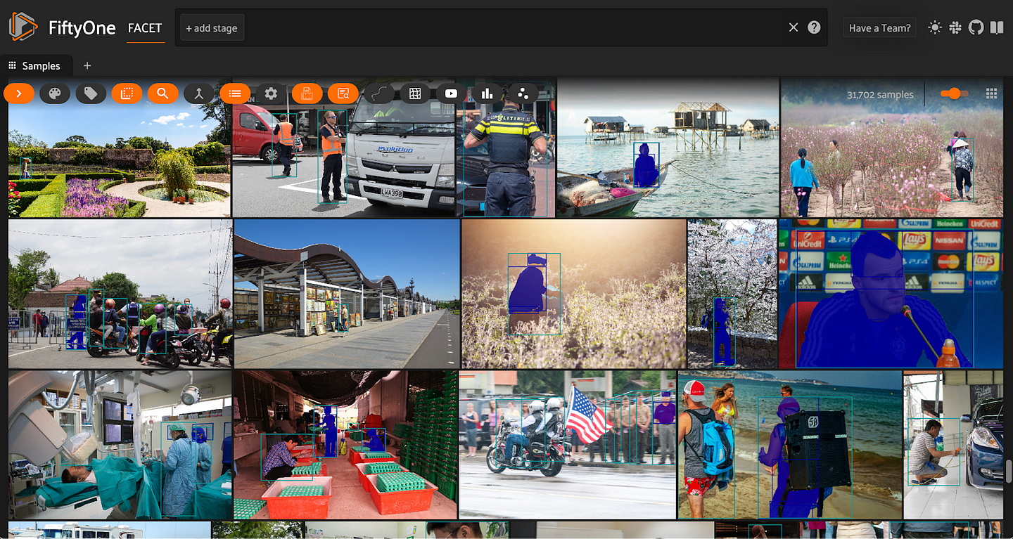
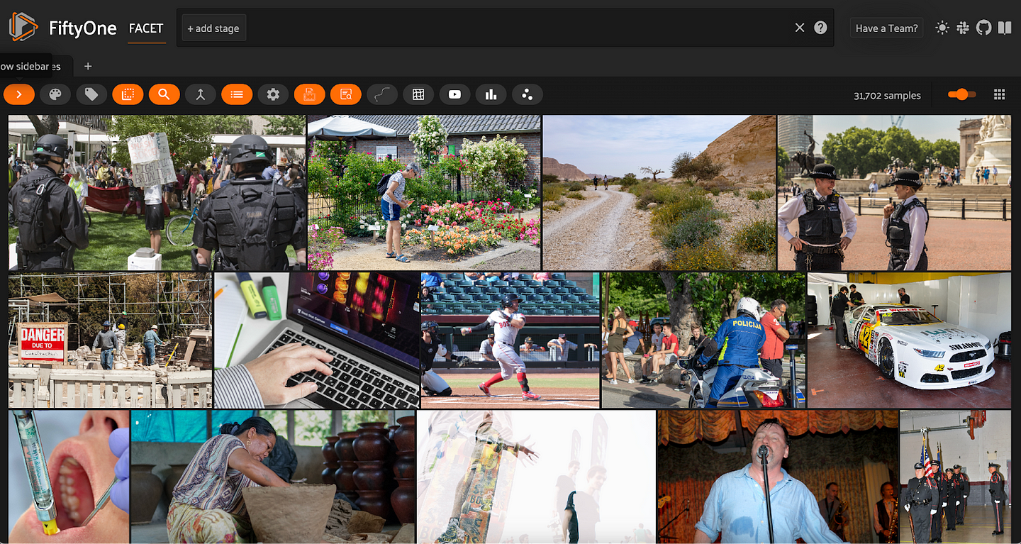
And we can launch a session of the FiftyOne App to view the images:

session = fo.launch_app(dataset)

Adding Person Detections

First, we load the ground truth annotations from CSV into a pandas DataFrame:

gt_df = pd.read_csv('annotations/annotations.csv')

Now we need to parse this DataFrame and add the appropriately structured data to our dataset. Like the authors of FACET do, let’s break things down into three types of attributes: 

1. Person attributes (hairtype, has_eyeware, etc.)
2. Protected attributes (perceived gender presentation, perceived age presentation, and perceived skin tone)
3. Other attributes (lighting, visibility)

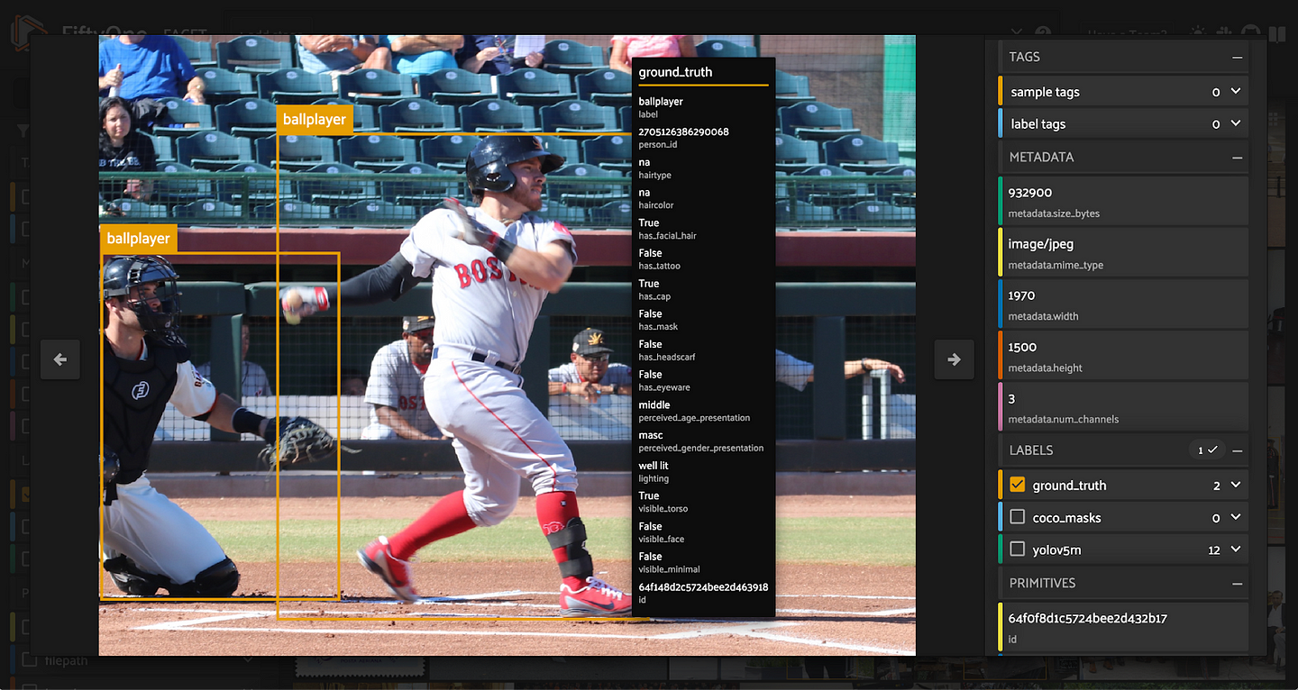
For each row in the dataframe, we will create a FiftyOne Detection, and we will add the relevant attributes to the detection.

Person attributes

We can create a tuple for the Boolean attributes we will iterate over:

BOOLEAN_PERSONAL_ATTRS = (
    "has_facial_hair",
    "has_tattoo",
    "has_cap",
    "has_mask",
    "has_headscarf",
    "has_eyeware",
)

def add_boolean_person_attributes(detection, row_index):
    for attr in BOOLEAN_PERSONAL_ATTRS:
        detection[attr] = gt_df.loc[row_index, attr].astype(bool)

We will also create some simple helper functions to restructure the hair type and color information:

def get_hairtype(row_index):
    hair_info = gt_df.loc[row_index, gt_df.columns.str.startswith('hairtype')]
    hairtype = hair_info[hair_info == 1]
    if len(hairtype) == 0:
        return None
    return hairtype.index[0].split('_')[1]

def get_haircolor(row_index):
    hair_info = gt_df.loc[row_index, gt_df.columns.str.startswith('hair_color')]
    haircolor = hair_info[hair_info == 1]
    if len(haircolor) == 0:
        return None
    return haircolor.index[0].split('_')[2]

All of this can be combined into a single function to add these person attributes:

def add_person_attributes(detection, row_index):
    detection["hairtype"] = get_hairtype(row_index)
    detection["haircolor"] = get_haircolor(row_index)
    add_boolean_person_attributes(detection, row_index)

Protected attributes

For perceived gender and perceived age, we will return whichever column with the associated prefix (“gender” or “age”) has a value of 1 in the given row. Aside from that, we just need to do a little string formatting.

def get_perceived_gender_presentation(row_index):
    gender_info = gt_df.loc[row_index, gt_df.columns.str.startswith('gender')]
    pgp = gender_info[gender_info == 1]
    if len(pgp) == 0:
        return None
    return pgp.index[0].replace("gender_presentation_", "").replace("_", " ")

def get_perceived_age_presentation(row_index):
    age_info = gt_df.loc[row_index, gt_df.columns.str.startswith('age')]
    pap = age_info[age_info == 1]
    if len(pap) == 0:
        return None
    return pap.index[0].split('_')[2]

For skin tone, a single detection might have multiple skin tones with nonzero values. To capture all of this information, we will just convert the skin tone columns into a dictionary and store the dictionary under a skin_tone attribute:

def get_skintone(row_index):
    skin_info = gt_df.loc[row_index, gt_df.columns.str.startswith('skin_tone')]
    return skin_info.to_dict()

Altogether, adding protected attributes to the detection is done in this function:

def add_protected_attributes(detection, row_index):
    detection["perceived_age_presentation"] = get_perceived_age_presentation(row_index)
    detection["perceived_gender_presentation"] = get_perceived_gender_presentation(row_index)
    detection["skin_tone"] = get_skintone(row_index)

Other attributes

As with the Boolean person attributes, we can create a tuple of visibility attributes to iterate over:

VISIBILITY_ATTRS = ("visible_torso", "visible_face", "visible_minimal")

Other than that, we just need to process the lighting information:

def get_lighting(row_index):
    lighting_info = gt_df.loc[row_index, gt_df.columns.str.startswith('lighting')]
    lighting = lighting_info[lighting_info == 1]
    if len(lighting) == 0:
        return None
    lighting = lighting.index[0].replace("lighting_", "").replace("_", " ")
    return lighting

def add_other_attributes(detection, row_index):
    detection["lighting"] = get_lighting(row_index)
    for attr in VISIBILITY_ATTRS:
        detection[attr] = gt_df.loc[row_index, attr].astype(bool)

Now we have all the pieces we need to create a Detection, given a row index from the pandas DataFrame. We will also pass the sample corresponding to that row in so that we can convert between absolute and relative bounding box coordinates:

def create_detection(row_index, sample):
    bbox_dict = json.loads(gt_df.loc[row_index, "bounding_box"])
    x, y, w, h = bbox_dict["x"], bbox_dict["y"], bbox_dict["width"], bbox_dict["height"]
    cat1, cat2 = bbox_dict["dict_attributes"]["cat1"], bbox_dict["dict_attributes"]["cat2"]

    person_id = gt_df.loc[row_index, "person_id"]

    img_width, img_height = sample.metadata.width, sample.metadata.height

    bounding_box = [x/img_width, y/img_height, w/img_width, h/img_height]
    detection = fo.Detection(
        label=cat1, 
        bounding_box=bounding_box,
        person_id=person_id,
        )
    if cat2 != 'none':
        detection["class2"] = cat2

    add_person_attributes(detection, row_index)
    add_protected_attributes(detection, row_index)
    add_other_attributes(detection, row_index)

    return detection

All that is left is to iterate over the samples in our dataset (this is more efficient than iterating over the rows in the gt_df DataFrame and filtering the dataset for the right sample), adding detections to each sample as we go:

def add_ground_truth_labels(dataset):
    for sample in dataset.iter_samples(autosave=True, progress=True):
        sample_annos = gt_df[gt_df['filename'] == sample.filename]
        detections = []
        for row in sample_annos.iterrows():
            row_index = row[0]
            detection = create_detection(row_index, sample)
            detections.append(detection)
        sample["ground_truth"] = fo.Detections(detections=detections)
    dataset.add_dynamic_sample_fields()

## add all of the ground truth labels
add_ground_truth_labels(dataset)

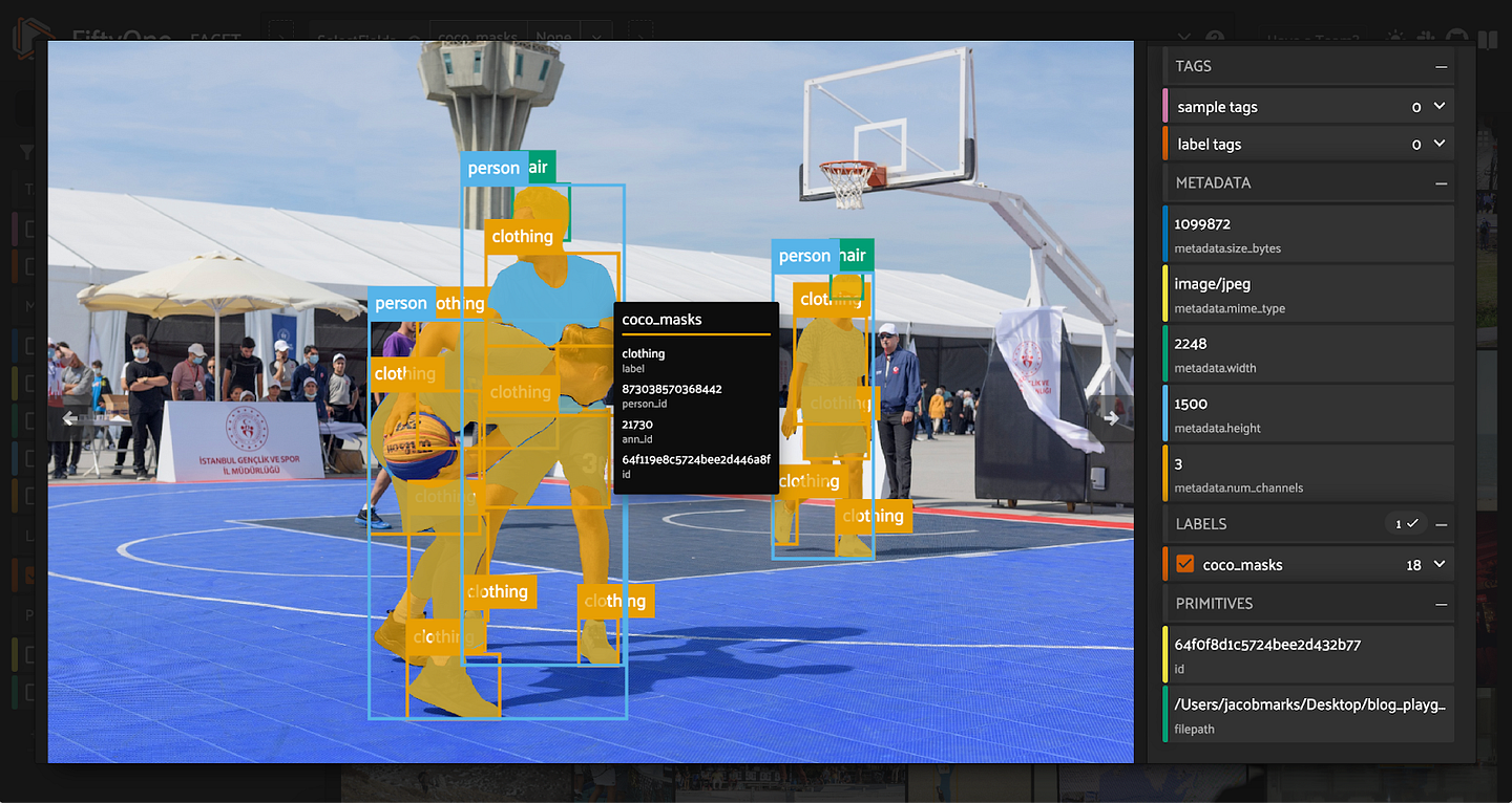
Adding Segmentation Masks

While the person, hair, and clothing segmentation masks are not strictly necessary for the detection and classification evaluation routines in the next section, it’s worth demonstrating how to add them, as the person masks can be used to evaluate instance segmentation models!

The add_coco_masks_to_dataset() function below does the following:

• Iterate through samples in the dataset
• For each sample whose filename has an entry in the COCO masks annotation file, we extract the segmentation mask and decode it from RLE format into a binary full image mask using pycocoutils.
• Using pillow and the bounding box associated with the segmentation mask, we crop the mask, turn it back into an array, and add the array as a mask (with bounding box) to a new Detection.

def add_coco_masks_to_dataset(dataset):
    coco_masks = json.load(open("annotations/coco_masks.json", "r"))
    cmas = coco_masks["annotations"]

    FILENAME_TO_ID = {
        img["file_name"]: img["id"]
        for img in coco_masks["images"]
    }

    CAT_TO_LABEL = {cat["id"]: cat["name"] for cat in coco_masks["categories"]}

    for sample in dataset.iter_samples(autosave=True, progress=True):
        fn = sample.filename

        if fn not in FILENAME_TO_ID:
            continue

        img_id = FILENAME_TO_ID[fn]
        img_width, img_height = sample.metadata.width, sample.metadata.height
        sample_annos = [a for a in cmas if a["image_id"] == img_id]
        if len(sample_annos) == 0:
            continue

        coco_detections = []
        for ann in sample_annos:
            label = CAT_TO_LABEL[ann["category_id"]]
            bbox = ann['bbox']
            ann_id = ann['ann_id']
            person_id = ann['facet_person_id']

            mask = maskUtils.decode(ann["segmentation"])
            mask = Image.fromarray(255*mask)

            ## Change bbox to be in the format [x, y, x, y]
            bbox[2] = bbox[0] + bbox[2]
            bbox[3] = bbox[1] + bbox[3]

            ## Get the cropped image
            cropped_mask = np.array(mask.crop(bbox)).astype(bool)

            ## Convert to relative [x, y, w, h] coordinates
            bbox[2] = bbox[2] - bbox[0]
            bbox[3] = bbox[3] - bbox[1]

            bbox[0] = bbox[0]/img_width
            bbox[1] = bbox[1]/img_height
            bbox[2] = bbox[2]/img_width
            bbox[3] = bbox[3]/img_height

            new_detection = fo.Detection(
                label=label, 
                bounding_box=bbox,
                person_id=person_id,
                ann_id=ann_id,
                mask=cropped_mask,
                )
            coco_detections.append(new_detection)
        sample["coco_masks"] = fo.Detections(detections=coco_detections)

## add the masks
add_coco_masks_to_dataset(dataset)

Evaluating Model Bias

FACET Evaluation Metrics

To evaluate your model biases using FACET, the dataset’s authors suggest looking at the recall of the model on subsets of the data defined by a concept and an attribute. For example, the concept could be a class label such as “backpacker”, and the attribute can be the value “curly” for hairstyle. Attributes can also be combined to explore prediction quality with intersectionality.

The model’s disparity in performance between two sets of attributes is the difference between its recall scores on these subsets.

When evaluating classification models (where classification is performed on the ground truth patches), the standard definition of recall is used:

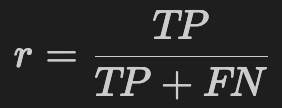
This can be interpreted as the rate at which true positives are correctly identified.

When evaluating detection models, only predictions with the person label are considered. Predictions are deemed correct when the overlap between ground truth bounding box and prediction bounding box — formally known as the Intersection over Union (IoU) — is greater than some threshold. The recall which is plugged into the disparity equation is the average recall over a sequence of IoU thresholds [0.5, 0.55, …, 0.95, 1.0], and is known as the mean average recall (mAR).

Adding Predictions to the Dataset

So that we can see these evaluation routines in action, let’s generate some predictions.

For detection, we’ll load YOLOv5m trained on COCO from the FiftyOne Model Zoo:

yolov5 = foz.load_zoo_model('yolov5m-coco-torch')

We can then apply the model to our dataset and store the predictions in a field on our samples with:

dataset.apply_model(yolov5, label_field="yolov5m")

### Just retain the "person" detections
people_view_values = dataset.filter_labels("yolov5m", F("label") == "person").values("yolov5m")
dataset.set_values("yolov5m", people_view_values)
dataset.save()

For zero-shot classification, as in the FACET paper, we will use a CLIP model with custom classes. We will again get the model from the FiftyOne Model Zoo:

## get a list of all 52 classes
facet_classes = dataset.distinct("ground_truth.detections.label")

## instantiate a CLIP model with these classes
clip = foz.load_zoo_model(
    "clip-vit-base32-torch",
    text_prompt="A photo of a",
    classes=facet_classes,
)

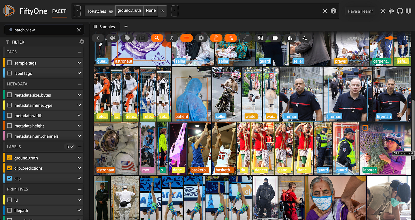
To generate classification predictions (effectively treating the ground_truth bounding box regions as their own images) we will use FiftyOne’s to_patches() method to create a view of all of the ground truth patches in our dataset, and then apply the CLIP model to these patches:

patch_view = dataset.to_patches("ground_truth")
patch_view.apply_model(clip, label_field="clip")
dataset.save_view("patch_view", patch_view)

The last line in the code block above saves this view to the dataset.

Evaluating Detection Predictions

Now that we have some detection and classification predictions, let’s write some code to compute the recall (or mean average recall) for a subset of the data. We will then illustrate how to filter for the subset corresponding to a specific concept and set of attributes.

For detections, we define the IoU thresholds we are going to average over:

IOU_THRESHS = np.round(np.arange(0.5, 1.0, 0.05), 2)

The following function only needs to be run once for each detection model:

def _evaluate_detection_model(dataset, label_field):
    eval_key = "eval_" + label_field.replace("-", "_")
    dataset.evaluate_detections(label_field, "ground_truth", eval_key=eval_key, classwise=False)
    
    for sample in dataset.iter_samples(autosave=True, progress=True):
        for pred in sample[label_field].detections:
            iou_field = f"{eval_key}_iou"
            if iou_field not in pred:
                continue

            iou = pred[iou_field]
            for it in IOU_THRESHS:
                pred[f"{iou_field}_{str(it).replace('.', '')}"] = iou >= it

This leverages FiftyOne’s built-in evaluate_detections() method to compute the IoU of each prediction bounding box that has overlap with a ground_truth bounding box. We pass in classwise=False because the labels for the ground truth detections are the 52 classes in the FACET dataset, whereas the label for our predictions is `person`. Which set of predictions to evaluate is specified by label_field.

After adding the IoU information to the predictions, we iterate over predictions, and store a Boolean for each IoU threshold, denoting whether or not the prediction would be considered a true positive at that threshold.

For any subset of the dataset — associated with a concept, attributes, or something else — we can compute the mean average recall as follows:

def _compute_detection_mAR(sample_collection, label_field):
    """Computes the mean average recall of the specified detection field.
    -- computed as the average over iou thresholds of the recall at
    each threshold.
    """
    eval_key = "eval_" + label_field.replace("-", "_")
    iou_recalls = []
    for it in IOU_THRESHS:
        field_str = f"{label_field}.detections.{eval_key}_iou_{str(it).replace('.', '')}"
        counts = sample_collection.count_values(field_str)
        tp, fn = counts.get(True, 0), counts.get(False, 0)
        recall = tp/float(tp + fn) if tp + fn > 0 else 0.0
        iou_recalls.append(recall)

    return np.mean(iou_recalls)

To close the loop with the FACET dataset, we can define a function, get_concept_attr_detection_mAR(), which takes in a concept (primary category for a person) and a dictionary of attributes in {field:value} form, and returns a mean average recall value for this combo:

def get_concept_attr_detection_mAR(dataset, label_field, concept, attributes):
    sub_view = dataset.filter_labels("ground_truth", F("label") == concept)
    for attribute in attributes.items():
        if "skin_tone" in attribute[0]:
            sub_view = sub_view.filter_labels("ground_truth", F(f"skin_tone.{attribute[0]}") != 0)
        else:
            sub_view = sub_view.filter_labels(f"ground_truth", F(attribute[0]) == attribute[1])
    return _compute_detection_mAR(sub_view, label_field)

As an example, let’s see YOLOv5m’s mean average recall for gymnasts with curly, black hair:

concept = 'gymnast'
attributes = {"hairtype": "curly", "haircolor": "black"}
get_concept_attr_detection_mAR(dataset, "yolov5m", concept, attributes)
## 0.875

This detection evaluation routine can be adapted into an instance segmentation evaluation routine by filtering the COCO masks down to just the person masks, and passing use_masks=True into evaluate_detections().

Evaluating Classification Predictions

In analog with detections, for classification models, we can create a _evaluate_classification_model() function which only needs to be run once per model:

def _evaluate_classification_model(dataset, prediction_field):
    patch_view = dataset.load_saved_view("patch_view")
    eval_key = "eval_" + prediction_field
    
    for sample in patch_view.iter_samples(progress=True):
        sample[eval_key] = (
            sample.ground_truth.label == sample[prediction_field].label
        )
        sample.save()
    dataset.save_view("patch_view", patch_view, overwrite=True)

This stores a True/False result on each sample in the patches view and saves this to the dataset.

Continuing the analogy with detections, we can compute classification recall for any collection of patches in the dataset:

def _compute_classification_recall(patch_collection, label_field):
    eval_key = "eval_" + label_field.split("_")[0]
    counts = patch_collection.count_values(eval_key)
    tp, fn = counts.get(True, 0), counts.get(False, 0)
    recall = tp/float(tp + fn) if tp + fn > 0 else 0.0
    return recall

And we can bring this back to subsets of our data described by concepts and attributes:

def get_concept_attr_classification_recall(dataset, label_field, concept, attributes):
    patch_view = dataset.load_saved_view("patch_view")
    sub_patch_view = patch_view.match(F("ground_truth.label") == concept)
    for attribute in attributes.items():
        if "skin_tone" in attribute[0]:
            sub_patch_view = sub_patch_view.match(F(f"ground_truth.skin_tone.{attribute[0]}") != 0)
        else:
            sub_patch_view = sub_patch_view.match(F(f"ground_truth.{attribute[0]}") == attribute[1])
    return _compute_classification_recall(sub_patch_view, label_field)

For the same concept-attributes combination from above, our CLIP model gives this:

get_concept_attr_classification_recall(dataset, "clip", concept, attribute)
## 0.6193353474320241

Assessing Disparity

For both detection and classification models, we can now compute the disparity between different sets of attributes for a shared concept.

We’ll create a get_concept_attr_recall() function, which will use the appropriate definition of recall depending on whether our label field houses classification or detection predictions:

def get_concept_attr_recall(dataset, label_field, concept, attribute):
    if label_field in dataset.get_field_schema().keys():
        return get_concept_attr_detection_mAR(dataset, label_field, concept, attribute)
    else:
        return get_concept_attr_classification_recall(dataset, label_field, concept, attribute)

And we will tie everything up in a nice bow with a compute_disparity() function:

def compute_disparity(dataset, label_field, concept, attribute1, attribute2):
    recall1 = get_concept_attr_recall(dataset, label_field, concept, attribute1)
    recall2 = get_concept_attr_recall(dataset, label_field, concept, attribute2)
    return recall1 - recall2

As an example, let’s look at the difference in CLIP model performance for some concepts when hair type is straight versus curly:

attrs1 = {"hairtype": "curly"}
attrs2 = {"hairtype": "straight"}

for concept in ["astronaut", "singer", "judge", "student"]:
    disparity = compute_disparity(dataset, "clip", concept, attrs1, attrs2)     
    print(f"{concept}: {disparity}")

#### OUTPUT ####
## astronaut: -0.8269230769230769
## singer: -0.0008051529790660261
## judge: -0.06666666666666667
## student: 0.16279069767441856

In the output, a value closer to +1 means that the model has higher recall for curly hair than straight hair, and a value closer to -1 means the model has a higher recall for straight hair. Whereas for singer, CLIP achieves roughly the same recall for people with straight hair and people with curly hair, there is a stark difference in performance for astronaut — CLIP has much higher recall for straight-haired astronauts than curly-haired astronauts.

You can also use FACET to compare models, combinations of attributes, and so much more!

Conclusion

There’s so much more to making a robust computer vision model than high mean average precision or F1 scores. Absent the appropriate caution and care, a model in production can exacerbate societal biases and even put people in physical danger.

The key to building a great model, in computer vision and machine learning more broadly, is to make the model truly serve all of the people who are impacted by the model’s predictions. The way to get there is diverse, high quality data, and rigorous evaluation. FACET makes it easier than ever to take steps to ensure that your models are equitable. There’s much more work to be done in order to make models fair to all, and we all need to play an active part in building an equitable future!