A Comprehensive Guide Using FiftyOne and Ultralytics YOLOv5
Drones are revolutionizing industries from agriculture to surveillance, and the ability to accurately detect and analyze objects from aerial imagery is becoming increasingly invaluable. Embarking on the journey of harnessing the potential of drone data through advanced object detection techniques is an exciting endeavor.
This tutorial dives deep into the powerful synergy between FiftyOne and Ultralytics YOLOv5, two cutting-edge tools that, when combined, offer a robust solution for training drone data. Whether you’re a seasoned machine learning practitioner or a drone enthusiast venturing into the realm of AI, this guide will equip you with the knowledge and tools to navigate the complexities of drone data training and object detection.
Wait, What’s FiftyOne?
FiftyOne is an open source machine learning toolset that enables data science teams to improve the performance of their computer vision models by helping them curate high quality datasets, evaluate models, find mistakes, visualize embeddings, and get to production faster.
Getting Started With Your Data
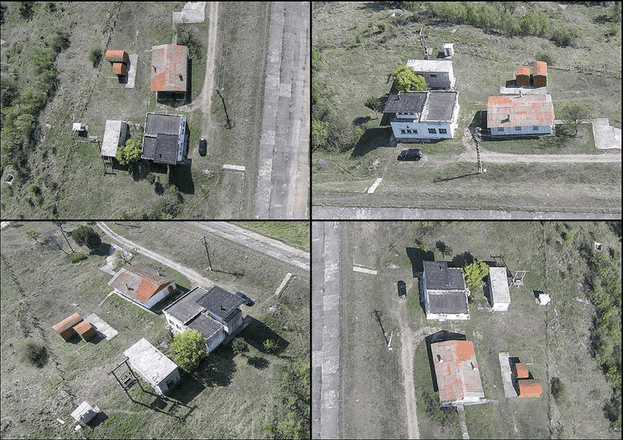
Drone data is very sensitive in computer vision and it is extremely important to keep all factors in mind. One small misrepresentation can severely hurt model accuracy. When curating or collecting data, it is important to take into account the angle, height, lens type, and more as to keep it consistent with how you plan on using your drone for its computer vision task. That task may be search and rescue, surveying, agriculture, or traffic detection. All of these tasks have different flight requirements and will be “seeing” the work it is doing differently.
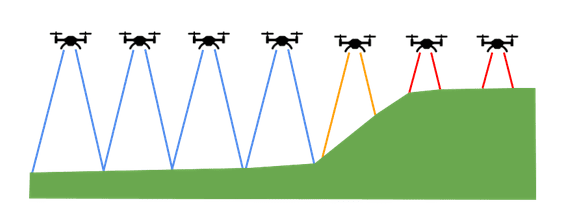
An easy to depict issue that can arise is the changing height of the terrain below the drone, which can lead to troublesome data. If there is an expected height above target for the use case, that should also be consistent on data collection. If the drone should be 50 feet above the ground but you are flying above a hill, the drone should also raise its altitude. Neglecting to do so will not only change the appearance of the image, but you can be missing coverage in your scan. None of these issues are going to totally impede training your model but could impact performance.
After all the data has been collected, the only actions you can make are additional annotations or data curation. Setting some guidelines for what data is acceptable and what is not for the use case is a great start.
For this walkthrough on using FiftyOne and Ultralytics to train an ML model on drone data, I will be using the Kaggle Roundabout Aerial Images dataset, but you can apply the same workflow to any annotated detection dataset though, so feel free to use your own.
Training With YOLOv5
One of the most painful experiences one goes through with training detection models is changing data types from one to another. Thankfully the days of parsing through several GB large COCO json files or scrambling together VOC xml files is over. FiftyOne allows you to natively convert your dataset to any type quickly and easily. We can start from data all the way to training in a few steps.
Step 1: Load Your Data
Let’s start by loading our VOC dataset.
import fiftyone as fo
import fiftyone.zoo as foz
import fiftyone.utils.random as four
import fiftyone.utils.yolo as fouy
from fiftyone import Dataset
from fiftyone.types import VOCDetectionDataset

# Path to the dataset directory
dataset_dir = "./original/original"

# Create a VOCDetectionDataset
dataset = Dataset.from_dir(
    dataset_dir,
    dataset_type=VOCDetectionDataset,
    label_field="ground_truth",
    name = "drone_original",
    overwrite=True
)
dataset.persistent =  True
Now that all of our data is loaded, it is time for us to convert it into into the YOLO format.
Step 2: Convert Into YOLO Format
To do this we will shuffle our data; we are using FiftyOne random_split. With it, we can easily split our data into a 85/15 split and export these datasets to the YOLO format. The operation will create a yaml file that points to the proper directories and will assist us in training. With these few steps, our data is already prepared to go train with Ultralytics!
four.random_split(dataset, {"val": 0.15, "train": 0.85})
val_view = dataset.match_tags("val")
train_view = dataset.match_tags("train")

val_view.export(
   export_dir="yolo_drone/",
   split="val",
   dataset_type=fo.types.YOLOv5Dataset,
)
train_view.export(
   export_dir="yolo_drone/",
   split="train",
   dataset_type=fo.types.YOLOv5Dataset,
)
Step 3: Training With Ultralytics
With our data all ready to go, next up is to train a model. Providing great tools as well as an extremely powerful model, Ultralytics is a great option when training your object detection models. To download, clone their YOLOv5 repository by running the commands in your terminal:
git clone https://github.com/ultralytics/yolov5  # clone
cd yolov5
pip install -r requirements.txt  # install
Ultralytics offers many different variations of training such as Multi-GPU, hyperparameter search, as well as pruning. For the sake of this demo, we will just be doing the default training. It is recommended that to achieve the highest accuracy you should tweak the training to fit your use case and data the best. For tutorials or tips on how to take advantage of YOLOv5 features, hop on over to their docs. For the default training, follow along with:
python3 /path/to/yolov5/train.py --data ./yolo_drone/dataset.yaml --weights yolov5s.pt --img 640
As is the case with most training runs, this can take quite a while on most machines and requires a graphics card. After the model has finished training and you are satisfied with the results, we can hop back into FiftyOne for some insights on how well the model trained.
Step 4: Post Training
Our model has been trained and our weights have been saved. Now, in order to deploy or run inference on our trained model, we need to export it to the format of our choosing. I chose TorchScript due to its fast compiled nature and ease to work with.
First locate your weights at /path/to/yolov5/runs/train/exp#/weights/best.pt then to export to Torchscript, run the following command:
python /path/to/yolov5/export.py --weights YOUR_WEIGHTS.pt --include torchscript
This will save the TorchScript file at the same location. The Ultralytics training run should have provided us with several evaluation marks such as loss or mAP. However, it is beneficial to take a deeper look to find exactly which images our model struggled with to develop a strategy to curtail this in future experiments. Let’s hop into FiftyOne for the answers!
Prepping the Model for Inference
import torch
import torchvision

#Load the Model
model = torch.load("/path/to/yolov5/runs/train/exp1/weights/best.torchscript")

#Define the Postprocessing Function
def non_max_suppression(
    	prediction,
    	conf_thres=0.25,
    	iou_thres=0.45,
    	classes=None,
    	agnostic=False,
    	multi_label=False,
    	labels=(),
    	max_det=300,
    	nm=0,  # number of masks
):
	"""Non-Maximum Suppression (NMS) on inference results to reject overlapping detections

	Returns:
        list of detections, on (n,6) tensor per image [xyxy, conf, cls]
	"""

	# Checks
	assert 0 <= conf_thres <= 1, f'Invalid Confidence threshold {conf_thres}, valid values are between 0.0 and 1.0'
	assert 0 <= iou_thres <= 1, f'Invalid IoU {iou_thres}, valid values are between 0.0 and 1.0'
	if isinstance(prediction, (list, tuple)):  # YOLOv5 model in validation model, output = (inference_out, loss_out)
    	prediction = prediction[0]  # select only inference output

	device = prediction.device
	mps = 'mps' in device.type  # Apple MPS
	if mps:  # MPS not fully supported yet, convert tensors to CPU before NMS
    	prediction = prediction.cpu()
	bs = prediction.shape[0]  # batch size
        nc = prediction.shape[2] - nm - 5  # number of classes
	xc = prediction[..., 4] > conf_thres  # candidates

	# Settings
	# min_wh = 2  # (pixels) minimum box width and height
	max_wh = 7680  # (pixels) maximum box width and height
	max_nms = 30000  # maximum number of boxes into torchvision.ops.nms()
	time_limit = 0.5 + 0.05 * bs  # seconds to quit after
	redundant = True  # require redundant detections
	multi_label &= nc > 1  # multiple labels per box (adds 0.5ms/img)
	merge = False  # use merge-NMS

	mi = 5 + nc  # mask start index
	output = [torch.zeros((0, 6 + nm), device=prediction.device)] * bs
	for xi, x in enumerate(prediction):  # image index, image inference
    	# Apply constraints
    	# x[((x[..., 2:4] < min_wh) | (x[..., 2:4] > max_wh)).any(1), 4] = 0  # width-height
    	x = x[xc[xi]]  # confidence

    	# Cat apriori labels if autolabelling
    	if labels and len(labels[xi]):
        	lb = labels[xi]
        	v = torch.zeros((len(lb), nc + nm + 5), device=x.device)
        	v[:, :4] = lb[:, 1:5]  # box
        	v[:, 4] = 1.0  # conf
        	v[range(len(lb)), lb[:, 0].long() + 5] = 1.0  # cls
      	x = torch.cat((x, v), 0)

    	# If none remain process next image
    	if not x.shape[0]:
        	continue

    	# Compute conf
    	x[:, 5:] *= x[:, 4:5]  # conf = obj_conf * cls_conf

    	# Box/Mask
    	box = xywh2xyxy(x[:, :4])  # center_x, center_y, width, height) to (x1, y1, x2, y2)
    	mask = x[:, mi:]  # zero columns if no masks

    	# Detections matrix nx6 (xyxy, conf, cls)
    	if multi_label:
        	i, j = (x[:, 5:mi] > conf_thres).nonzero(as_tuple=False).T
        	x = torch.cat((box[i], x[i, 5 + j, None], j
                     mask[i]), 1)
    	else:  # best class only
        	conf, j = x[:, 5:mi].max(1, keepdim=True)
        	x = torch.cat((box, conf, j.float(), mask), 1)[conf.view(-1) > conf_thres]

    	# Filter by class
    	if classes is not None:
        	x = x[(x[:, 5:6] == torch.tensor(classes, device=x.device)).any(1)]

    	# Apply finite constraint
    	# if not torch.isfinite(x).all():
    	# 	x = x[torch.isfinite(x).all(1)]

    	# Check shape
    	n = x.shape[0]  # number of boxes
    	if not n:  # no boxes
        	continue
    	x = x[x[:, 4].argsort(descending=True)[:max_nms]]  # sort by confidence and remove excess boxes

    	# Batched NMS
    	c = x[:, 5:6] * (0 if agnostic else max_wh)  # classes
    	boxes, scores = x[:, :4] + c, x[:, 4]  # boxes (offset by class), scores
    	i = torchvision.ops.nms(boxes, scores, iou_thres)  # NMS
    	i = i[:max_det]  # limit detections
    	if merge and (1 < n < 3E3):  # Merge NMS (boxes merged using weighted mean)
        	# update boxes as boxes(i,4) = weights(i,n) * boxes(n,4)
        	iou = box_iou(boxes[i], boxes) > iou_thres  # iou matrix
        	weights = iou * scores[None]  # box weights
        	x[i, :4] = torch.mm(weights, x[:, :4]).float() / weights.sum(1, keepdim=True)  # merged boxes
        	if redundant:
            	i = i[iou.sum(1) > 1]  # require redundancy

    	output[xi] = x[i]
    	if mps:
        	output[xi] = output[xi].to(device)

	return output

def xywh2xyxy(x):
	# Convert nx4 boxes from [x, y, w, h] to [x1, y1, x2, y2] where xy1=top-left, xy2=bottom-right
	y = x.clone() if isinstance(x, torch.Tensor) else np.copy(x)
	y[..., 0] = x[..., 0] - x[..., 2] / 2  # top left x
	y[..., 1] = x[..., 1] - x[..., 3] / 2  # top left y
	y[..., 2] = x[..., 0] + x[..., 2] / 2  # bottom right x
	y[..., 3] = x[..., 1] + x[..., 3] / 2  # bottom right y
	return y

def format_detections(preds):
	detections = []
	for x in preds:
        	label = x[5].cpu().detach().numpy()
        	score = x[4].cpu().detach().numpy()
        	box = x[:4].cpu().detach().numpy()
        	x1, y1, x2, y2 = box
        	rel_box = [x1 / w, y1 / h, (x2 - x1) / w, (y2 - y1) / h]
        	detections.append(
        	fo.Detection(
            	label=classes[int(label)],
            	bounding_box=rel_box,
           	confidence=score
        	)
    	)
	return detections
With our model loaded and ready to go, let’s take a slice of our dataset and introspect a bit. We start with creating a prediction view of 100 samples:
predictions_view = dataset.take(100, seed=51)
We follow up by creating an inference loop that will inference on the 100 images and add the detections to the samples. This will allow us to compare the detections in the FiftyOne App in the future.
from PIL import Image
import cv2
from torchvision.transforms import functional as func

device = "cuda"
classes = ["vehicle", "cycle", "truck", "bus", "van"]
model = model.to(device)


with fo.ProgressBar() as pb:
	for sample in pb(predictions_view):
    	# Load image
    	image = cv2.imread(sample.filepath)
    	image = cv2.resize(image, (640, 640))
    	image = func.to_tensor(image).to(device)
    	c, h, w = image.shape
    	#pint(image.shape)

    	# Perform inference
    	preds = model(image.unsqueeze(0))
    	out = non_max_suppression(preds)
    	detections = format_detections(out[0])
    	# Save predictions to dataset
    	sample["yolov5"] = fo.Detections(detections=detections)
    	sample.save()

session.view = predictions_view
With the App restarted and our new view in place, we can extract fresh insights from our data. Immediately, we’re able to observe our detections superimposed on the ground truths, facilitating a performance evaluation. Additionally, the option to hide the ground truths provides a clear picture of missed detections. Another valuable suggestion is to experiment with the label confidence sliders, offering a glimpse of our high and low-confidence predictions.
Upon analyzing the data, I can draw conclusions that were previously inaccessible without a thorough examination:
- The model performs strongly with high confidence on cars going around the roundabout
- The model struggles at closely bunched cars, such as parked cars
- The model mistakes rectangular objects as vehicles potentially
Investigating the Embeddings
With the FiftyOne Brain, we can take an even deeper look at our data and predictions by using embeddings. By executing a couple commands beforehand, we can open a power visualization tool that shows the groups within your data and how your model is performing on them. Take a look below:
import fiftyone.brain as fob

#Grab the mAP and IoUs
results = predictions_view.evaluate_detections(
	"yolov5",
	gt_field="ground_truth",
	eval_key="eval",
	compute_mAP=True,
)

#Compute ground_truth embeddings
results = fob.compute_visualization(
	predictions_view, patches_field="ground_truth", brain_key="gt_viz"
)

#Compute yolov5 embeddings
results = fob.compute_visualization(
	predictions_view, patches_field="yolov5", brain_key="yolo_viz"
)

session.view = predictions_view
We can grab awesome insights of where maybe we need to add to our dataset. We can potentially try to add more parked car views, different street views other than roundabouts, or even think about decreasing the height of the drone to increase the information we get about each car. Looking through our highest and lowest confidence predictions compared to ground truths allows us to learn more about data than a simple training run or evaluation could ever do.
If you’d like learn more, check out this talk I gave about many of the topics in this blog in August at the Computer Vision Meetup.
In summary, this tutorial has explored the exciting realm of harnessing the potential of drone data, spotlighting the synergy between FiftyOne and Ultralytics YOLOv5. By meticulously curating drone data and leveraging these powerful tools, this guide equips both AI enthusiasts and machine learning practitioners with the expertise to navigate the complexities of object detection training. The provided steps, from data preparation and model training to post-training analysis, underscore the importance of tailored approaches for specific use cases of working with drone data. By offering insights into model performance and utilizing embeddings for deeper analysis, this tutorial empowers users to drive accuracy and make informed decisions in the dynamic intersection of drone technology and artificial intelligence.

