Why a 3D Corgi From a Year Ago Is More Profound Than You Think
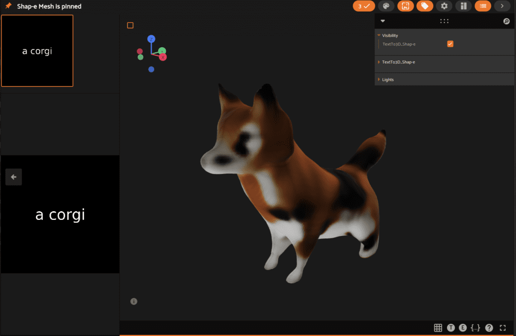
Diffusion models are generative AI models that have skyrocketed in popularity in the last few years. Inspired by non-equilibrium equations in thermodynamics, diffusion is trained to denoise a sample. Diffusion models come in many flavors, from OpenAI’s DALLE or Stability AI’s Stable Diffusion, but these models focus on image samples. To tackle 3D samples, OpenAI researchers must rethink how we use diffusion models. Now, a year after the release of Shap-E, we can look back and see how incredible the journey was.
How Does Diffusion Work?
Before we understand what makes Shap-E so profound, let’s look at diffusion as a whole. Disclaimer: I will quickly breeze through the main foundation of today’s diffusion models and might make some oversimplifications 🤷♂️. The history of diffusion could be a whole blog on its own so we will keep it short. If you are interested in diving deeper into a topic of diffusion I mentioned, I’ve included links to the sources. Now, let’s jump into it!
Diffusion, at its core, is the act of modeling the way noise “diffuses” through the entire dataset. Once the model understands how the noise diffuses, one can reverse the process, allowing it to take a random sample and denoise it until it recreates the target sample. In other words, diffusion has two main parts: the forward and reverse process. The forward process is about adding noise to destroy a sample, and the reverse process is about trying to recreate the original sample from the noise. The forward diffusion process is described by the equation below:

Reading left to right, the equation starts with , where
defines the forward process,
is the output at step
and
is the input for the process. On the right
is a normal distribution where we add noise with the mean
and variance of
. In this equation
is the schedule, and its values range between 0 and 1. The schedule’s job is to keep the variance from exploding and it allows us to gradually add noise to the sample over time. Looking at the big picture, we now have a function where we can find at any time step the amount of noise to add and as
, we will have created an entirely random sample. Perfect! Now that we can show a model how a sample goes from original to random, we can train the model to reverse the process, and go from random to a generated sample!
But wait, how can we just reverse the process? Why does this work in the first place? Eventually, over time, we can teach the model the structure of our data, what an edge is, for instance, and how edges tend to meet in our samples. The model is able to abstract out the structure of our data to high levels to where it is then able to recreate it in the reverse process, because of its strong priors.
Now, some great math happens before the equation above can be reversed effectively, but it’s a bit out of the scope of this blog. The 2020 paper, Denoising Diffusion Probabilistic Model, took a giant stride by defining the equations in a way that could be easily modeled. OpenAI’s 2021 paper, Improved Denoising Diffusion Probabilistic Models, improved it further with modification to the schedule and reduction to the overall Gaussian noise. Both are great reads if you are interested in the development of the models. I will briefly summarize the reverse process.

The reverse process as shown in DDPM
Above is a diagram that visualizes the forward and reverse process of diffusion. We use the forward process, , to add noise to a sample until time step
. Afterwards, we use the reverse process to approximate all the noise that is to be removed from the noisy sample
to recreate the original sample
.
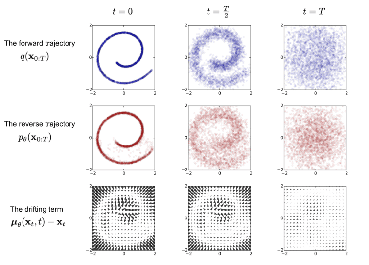
Diagram showing how samples are deconstructed and reconstructed with diffusion
Slowly over time, we increase the amount of noise that can be removed from each step with the same schedule, , until the final step, where we take the full amount and don’t add any extra noise between steps. Finally, we arrive at our formula for predicting the next step in the reverse process:

Calculate the output at any time step t
In this case, our model is predicting , the noise to be removed. With a process in place, we can now begin training a model to predict it!
Developments in Diffusion
Diffusion model architecture (when I say model from here on out, I am referring to the ML model predicting the noise) can vary from one paper to the next. Many have used attention blocks and U-Nets to great effect with many variations in training methods, datasets, and more. Instead of focusing on small nuances, I will cover all the main developments in how we think about diffusion today and why Shap-E is a culmination of a decade of research. To sum up diffusion training briefly, it goes something like this ⬇️:
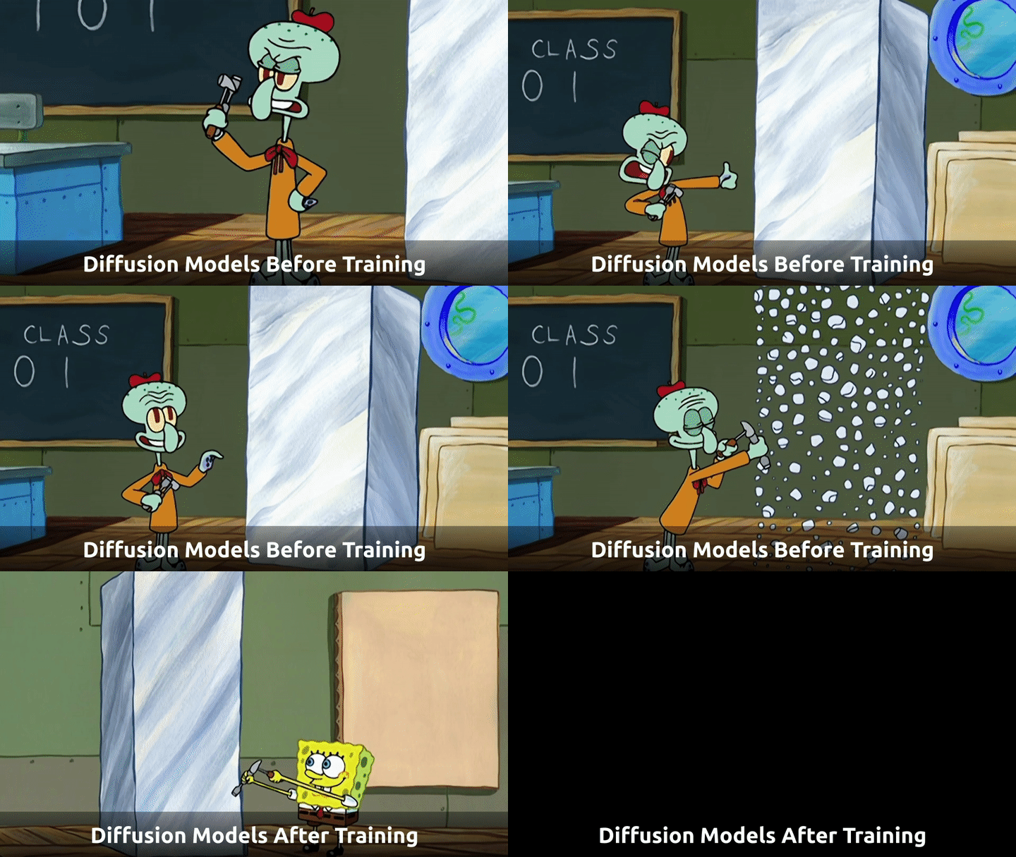
Models attempt to recreate the original and then are scored on the reconstruction’s performance. Weights are trained based on the error, and the cycle continues until the reconstructions are refined. Remember that the goal at this point is only the reconstruction of a sample. Diffusion was locked in on seeing who could best denoise an image. So what changed?
Classifier Guided Diffusion
The first major improvement since the DDPM paper, in Dhariwal and Nichol 2021, the authors proposed adding a classifier to the process that would help guide the model to a better reconstruction. If the model classified the image as a dog or a cat, it would guide the reconstruction accordingly based on the classification. After the adoption of the U-Net as the best backbone at the time and some squabbling over training parameters to get to the best performance, a new approach was taken and the process was altered by adding another component. The authors showed that by adding classifier guidance, reconstruction greatly improved.
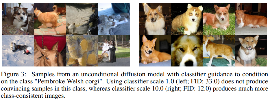
Figure from Dhariwal and Nichol 2021
Below, we see the modified noise predictor, , which has the added class guidance component.

While this was not the first conditioning done on a diffusion model (Song et al. previously performed score-based conditioning), it was the first time a diffusion model was conditioned on additional information outside of the image. Never before had diffusion been guided in a specific direction, and the results were extremely promising.
Classifier-Free Guided Diffusion
The next major advancement by Ho and Salimans in 2021 was creating a diffusion model that can both use a classifier and ignore it in one architecture. Through training and randomly throwing away some of the conditionings at training time, classifier-free guided diffusion created a model that performs strongly on both guided and unguided tasks. Classifier-free guidance had the additional benefits of simpler training, no increase in parameters, and no need for a classifier/a noisy dataset to train the classifier
Even more important for future considerations, having a dual guided+unguided setup made the model much less susceptible to adversarial activities. If you knew the classifier’s weakness, you could expose it in the diffusion model. By having both streams, the model could handle more diverse samples while maintaining a good reconstruction score.
Latent Diffusion
The final piece of the puzzle was latent diffusion. Rombach et al. propose in High-Resolution Image Synthesis with Latent Diffusion Models a “departure to latent space.” By dropping the dimensionality of the input sample using an autoencoder, we can define a latent space in which the diffusion happens. This small change to move away from image compression like in past works and make use of latent spaces drastically improved model efficiency. Latent space now allowed models to encode the important representational information better, while ignoring the noise of pixel values. Predictions came out faster, and transferring to latent spaces allowed the model to increase its overall training capacity due to the new efficiencies.
Even more important than the efficiency improvements, diffusion had become multi-modal. CLIP crashed onto the scene and became the gold standard of transferable vision models. There was now a connection between text and images through the new latent space that was created. The autoencoder that creates the latent space is also completely modular, meaning a single autoencoder model can be used for many different diffusion model architectures. The changes allowed tasks performed with latent diffusion, like super-resolution or text-to-image, to rocket past its competitors in other architectures like GANs. We were no longer just recreating samples, but pushing them conceptually in a direction we determined.
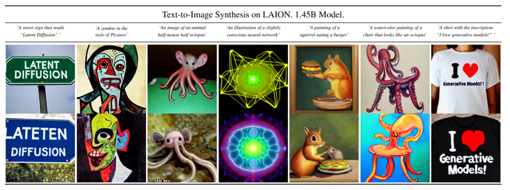
Early Text-To-Image Results from Rombach et al. 2022
The model created from this paper would later become known as Stable Diffusion. From there it was off to the races to see who could make the best model. OpenAI would answer back soon after with DALL-E 2, using CLIP encodings as their latent space. From there, Stability.ai and OpenAI would go back and forth, incrementally improving their text-to-image models. This is a blog about Shap-E though, so what happened to make it so special?
Crossing into New Territory with 3D Generation
It is fair to say that the images generated by latent diffusion text-to-image models are incredible, and the rate at which the models have improved from 2020 to now is astonishing. However, one part was still missing on the math/theoretical side. While latent diffusion marked the departure to latent space, the destination was still a pixel world. Despite all the advancements, most of the work had one goal: reconstructing an image. If diffusion models aim to solve additional complex, real-world modeling problems, they must depart from pixel space.
Shap-E takes the existing latent diffusion model and improves upon it by targeting an implicit neural representation (INR), a powerful tool to encode continuously a variety of different signals like images, videos, audio and 3D shapes. In the case of Shap-E the two INRs they targeted were NeRFs and DMTet or its extension GET3D. The latter two are also known as 3D meshes.

An example of a NeRF
Instead of targeting the reconstruction of a 2D sample, Shap-E targets an INR that represents a 3D object. INRs also have the unique property of being continuous and end-to-end differentiable compared to other previous 3D encodings. Hold that thought as we continue to explore Shap-E.
Shap-E aims to create a model that can take in text or an image to generate a new 3D object. Like before, the diffusion model uses CLIP embeddings to define their latent space on the input. They also support classifier-free guidance by randomly setting the conditioning information to zero during training with a probability of 0.1. Most importantly, they choose not to predict the noise to be removed but to sample directly. In theory, predicting the noise to be removed is equivalent to predicting the post-noise-removal state directly. In practice, the latter approach produces more coherent results.

Reconstruction of Noised Latents
The Legacy of Shap-E
With Shap-E, OpenAI accomplished their goal of creating a diffusion model that could take in an image or text and output a 3D object. If you are wondering what that looks like, I’ve included results from the paper below⬇️:
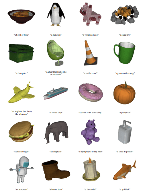
Admittedly, they are not the highest quality. But that shouldn’t be the takeaway here because there was a more significant achievement. Shap-E could take in a latent space of two separate modalities to generate a prediction for targeting not one but two different INRs. That means we could describe a latent space that could be learnt to estimate a differential function! The model follows below to estimate the underlying continuous function :

The network parametrizes the variable and then implicitly encodes the estimate function
into the network, hence the name “implicit neural representation.” No longer are diffusion models bound by pixels. We can express problems in any field if we can model the function to fit the diffusion model! We can even transfer different encoders from multiple modalities to pair with diffusion architectures for endless other modalities.
Diffusion models have contributed greatly to computational protein design and generation, drug and small-molecule design, protein–ligand interaction modeling, cryo-electron microscopy data enhancement, and single-cell data analysis. We are seeing chemists model molecule generation with guided diffusion. Diffusion models are even being used to predict the weather.
Shap-E was only possible through a decade of tremendous research. But it also serves as a departure point for diffusion models from just image denoising and generation to something much greater. The next vaccine, breakthrough in molecular biology, or other scientific innovation could very well owe in part to a diffusion model. Diffusion has become just that good.
Explore Diffusion Models
Phew, that was a long history. Now it’s time to have fun and explore. To access some diffusion models, including new ones like Stable Diffusion 3 and Stable Video Diffusion, you must leverage a model-serving API like fireworks.ai or OpenAI’s API. Older models like Shap-E are open source and can be found on GitHub.
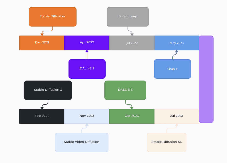
Timeline of Diffusion Models Over the Years
I’ll walk through how we can compare many of the popular diffusion models, all in one place. Let’s start with the easiest use case, text-to-image.
Text to Image Diffusion
To compare our images in one place, we will use the FiftyOne Python library, a tool for managing your computer vision datasets. From there, we can leverage a plugin that has included many popular text-to-image models. Here is how we can get started:
pip install fiftyone
fiftyone plugins download https://github.com/jacobmarks/text-to-image
As mentioned, many of these diffusion models are best run on a model-serving platform due to hardware strain or availability. Below is the breakdown of where to get these models and how we can run them:
Many of these models cost less than a cent to run and deliver fast inference results! They are extremely convenient to use and flexible. If you are interested in using them, sign up and make sure to add your API key to your environment key before moving on:
# Replicate
pip install replicate
export REPLICATE_API_TOKEN=######

# OpenAI
pip install openai
export OPENAI_API_KEY=########

# StabilityAI
pip install requests
export STABILITY_API_KEY=######
After we have installed the required dependencies, we want to create a dataset to hold our new text-to-image results. It will be empty to start, but we will quickly fill it. To create a dataset and launch the visualization app in a new tab, open up a notebook and run the following code:
import fiftyone as fo

dataset = fo.Dataset("Text-to-Image")
session = fo.launch_app(dataset)
From here, we can browse operations and find the text-to-image operator using backtick, “ ` “. Select the model you want to run and enter your preferred inputs, including a prompt. After a second or two, your new image will be loaded into the app!
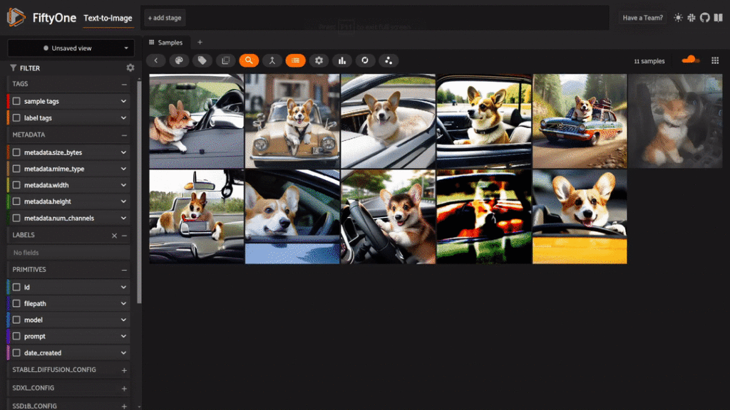
We can leverage this plugin to compare multiple models across a single prompt and explore tuning input parameters like the number of steps, image size, and more. Let’s take a look at how responses from a simple prompt like “a corgi driving a car” have changed over the years:
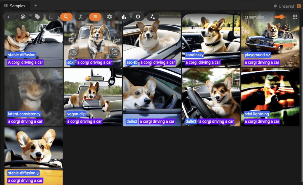
Different Outputs from the Same Prompt
There are many interesting takeaways from trying a single prompt across all models, but I was personally really surprised by how great the results were from models that don’t come first to your mind. Playground-v2 and Kandinsky both have sharp images that nail the context of a corgi driving a car. Playground even seems to have its own style. It is also one of only two models that shows a full car and the only one where the car seems to be moving! Much of this is dependent on how you craft your prompts, too, so be careful and try different options!
Stable Video Diffusion
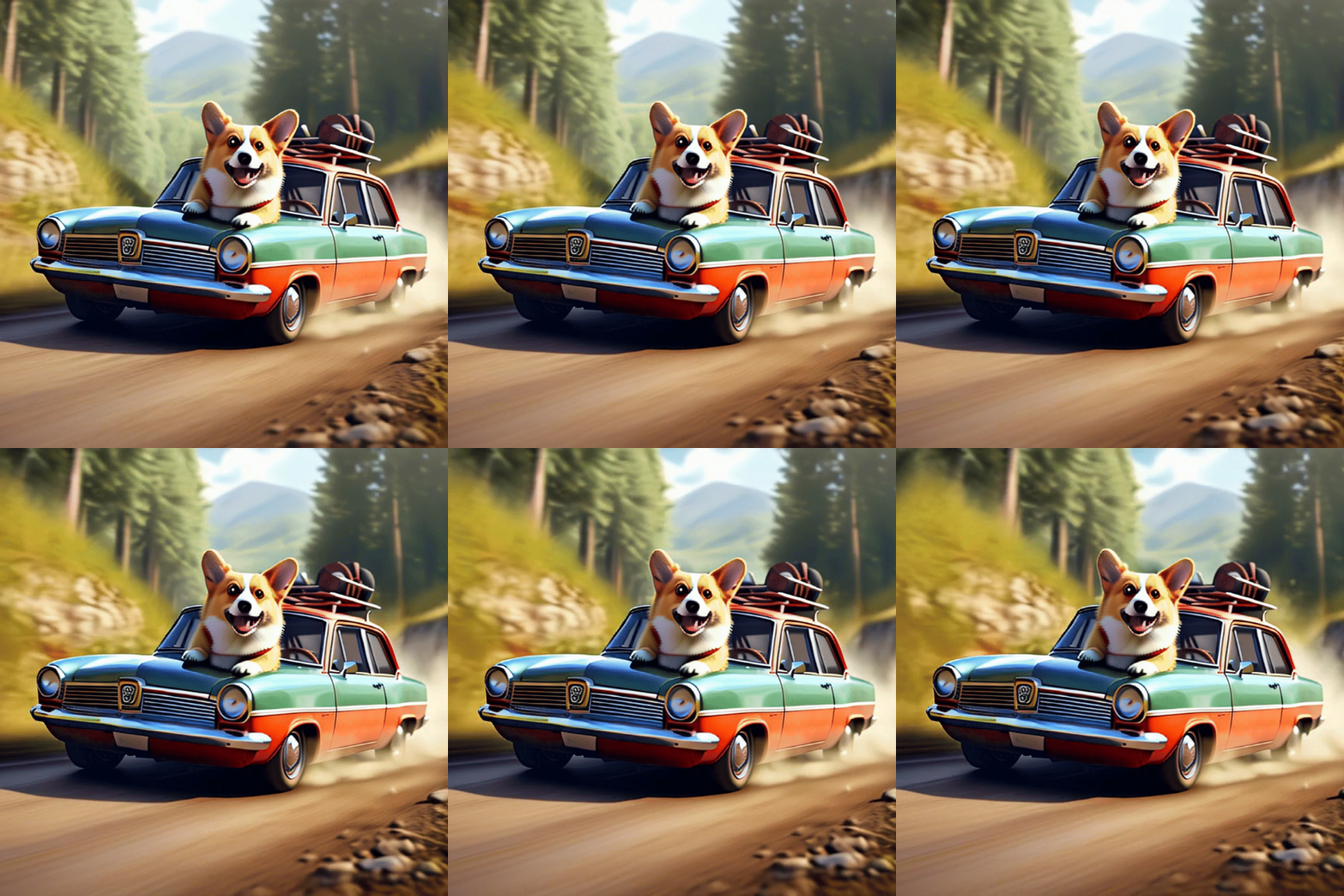
One of the more recent developments in diffusion models has been for the task of image-to-video. Stability.ai released its stable video diffusion for non-commercial use several months ago. We can take one of our samples from text-to-image and take it an extra step with image-to-video! We will use a replicate model again and use the image-to-video plugin to test out the model!
fiftyone plugins download https://github.com/danielgural/img_to_video_plugin
Afterwards, we can select the image we would like to animate and call the operator `img2video` by opening up the operators list with the “ ` “ key or by selecting the operators button. Send the image in and soon, a new dataset will be created called img2video with the results!
Text/Image to 3D Diffusion with Shap-E
Finally, we reached the star of the day, Shap-E! We can explore the task of 3D object generation with both text-to-3D and image-to-3D. To get started, we need to grab a plugin that will do the heavy lifting for us.
fiftyone plugins download https://github.com/danielgural/shap_e_plugin
pip install diffusers
With Shap-E we are able to transform any text prompt or image directly into a 3D mesh. Let’s check out some examples! Open the app like so to get started:
import fiftyone as fo

session = fo.launch_app()
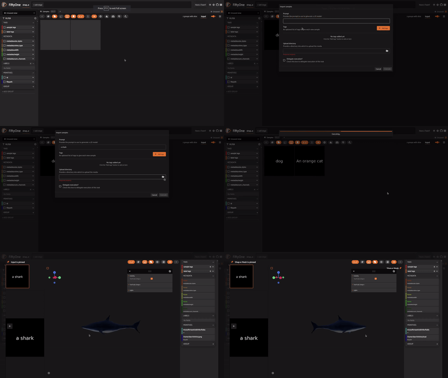
Text to 3D
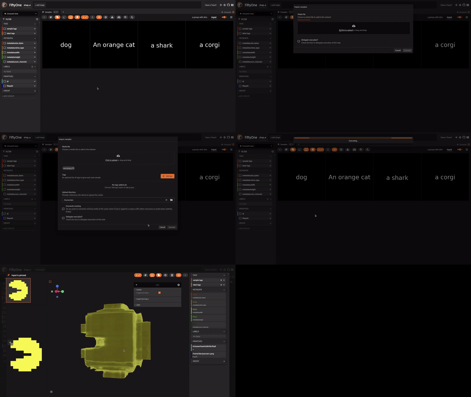
Image to 3D
What’s Next?
It is mind-boggling how much diffusion models have advanced in the last two years. Even in 3D, new models like InstantMesh can deliver stunning image-to-3D results, with quality much higher than that of the only year-old Shap-E model. The anticipation of seeing what diffusion model will come next is thrilling, and the prospect of applying diffusion to other fields like medicine, biology, chemistry, and more is exhilarating. Who knows what answers are just waiting to be unlocked?

