How to make sense of the model outputs and parse them into FiftyOne format

Source: CoTracker3 Website

CoTracker3 is designed to track individual points throughout a video sequence. Given a video and the initial location of a point in a specific frame, it predicts that point’s trajectory over time, even when the point is occluded or moves out of the camera’s view.

What makes CoTracker3 stand out from other point trackers’ ability to effectively leverage real-world videos during training, resulting in SOTA performance on the point tracking task.

Most SOTA point trackers rely heavily on synthetic datasets for training due to the difficulty of annotating real-world videos. CoTracker3 overcomes this limitation using a semi-supervised training approach incorporating unlabeled real-world videos. This is achieved by employing multiple existing point trackers (trained on synthetic data) as “teachers” to generate pseudo-labels for the unlabeled videos.

CoTracker3, as the “student,” then learns from these pseudo-labels, effectively bridging the gap between synthetic and real-world data distributions. This strategy allows CoTracker3 to achieve SOTA accuracy on benchmark datasets while being trained on less real-world training data than previous methods.

I highly recommend reading the paper if you’re interested in all the nitty gritty details. In this post, we’re hands-on. I’ll show you how to run inference with the model and parse the output into FiftyOne format.

👨🏽‍💻 Let’s code!

Note: you can jump right into the Google Colab notebook or clone the repo and run it locally (assuming you have a GPU with enough RAM)

Start off with installing the required libraries:

pip install fiftyone imageio[ffmpeg]

Let’s download a dataset. I’ve got one here on Hugging Face you can download:

import fiftyone as fo
from fiftyone.utils.huggingface import load_from_hub

dataset = load_from_hub("harpreetsahota/videos-to-test-trackers")

You can do an initial exploration of the dataset using the FiftyOne app:

fo.launch_app(dataset)

There are a couple of ways you can use the model. One is cloning the CoTracker GitHub repository using the code there. The other is to download the model from the Torch hub. The model comes in two flavours: online and offline.

Online and Offline Modes in CoTracker3

Both online and offline versions of CoTracker3 have the same model architecture.

The difference is their training procedures and how they utilize temporal information at inference, specifically how they process the input video and the direction in which they track points.

CoTracker3 Online: Processes the video sequentially in a sliding window. It tracks points forward-only, making predictions based on previously seen frames. This mode enables real-time tracking for an indefinite duration, limited only by computational resources.

CoTracker3 Offline: Processes the entire video simultaneously as a single sliding window. This allows tracking points bidirectionally, leveraging information from both past and future frames. The offline has better performance, especially for tracking occluded points. This is because it interpolates trajectories through occlusions using the entire video context.

However, unlike the online version, the maximum number of frames it can process is limited by memory.

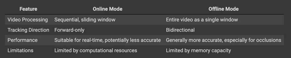
Online vs offline mode for CoTracker3

I’ll use the offline mode for this tutorial. You can download the model like so:

import torch

device = "cuda" if torch.cuda.is_available() else "cpu" #highly recommend using a GPU

cotracker = torch.hub.load("facebookresearch/co-tracker", "cotracker3_offline").to(device)

Let’s prepare a video for inference using the model.

import imageio
import numpy as np
from IPython.display import HTML
from base64 import b64encode

def read_video_from_path(path):
    """
    Read a video file and convert it to a tensor.
    
    Args:
        path (str): Path to the video file
    
    Returns:
        torch.Tensor: Video tensor of shape (1, num_frames, 3, height, width)
    """
    reader = imageio.get_reader(path)
    frames = [np.array(im) for im in reader]
    # Stack frames, convert to torch tensor, and rearrange dimensions
    return torch.from_numpy(np.stack(frames)).permute(0, 3, 1, 2)[None].float()

def show_video(video_path):
    video_file = open(video_path, "r+b").read()
    video_url = f"data:video/mp4;base64,{b64encode(video_file).decode()}"
    return HTML(f"""<video width="640" height="480" autoplay loop controls><source src="{video_url}"></video>""")

video_path = dataset.values("filepath")[1]

show_video(video_path)

From Pexels.com

And we can load this video as a tensor:

video_tensor = read_video_from_path(video_path)

The model accepts a tensor with the following shape: B T C H W. Where B is the batch size, T is the number of frames, C is the number of input channels, H is the video height and W is the video width.

Let’s confirm the shape of the tensor:

video_tensor.shape 
# torch.Size([1, 62, 3, 3840, 2160])

Before running inference, let’s move the model and video to the GPU:

if torch.cuda.is_available():
    model = cotracker.cuda()
    video = video_tensor.cuda(

The grid_size parameter in CoTracker3 determines the number of points in a grid that will be tracked within a video frame. It offers a way to specify the density of tracked points across the video frame when you don’t have specific points you want to track

• When grid_size is greater than 0, the model computes tracks for a grid of points on the first frame. The grid will have grid_size * grid_size points.
• This parameter is used in conjunction with queries and segm_mask.
• If queries is not provided, and grid_size is set, the model will track points on a regular grid.
• If a segm_mask is also provided, the grid points are computed only for the masked area.

Larger grid_size values consume more GPU memory.

When you increase the grid_size in the CoTracker model, it leads to higher GPU memory consumption.

• The grid_size parameter determines the number of points that the model tracks. A larger grid_size means more points are being tracked, which requires more memory to store and process their information. If you find yourself encountering out-of-memory errors, consider reducing the values of grid_size
• CoTracker uses a grid of points overlaid on the video frames. A larger grid_size results in more dense feature maps, which require more memory to compute and store.
• With more points to track, the model needs to perform more computations, which can lead to increased memory usage for intermediate results and gradients (even though we’re using torch.no_grad()).

We can run inference as follows:

with torch.no_grad():
  pred_tracks, pred_visibility = model(video, grid_size=20)

Examining the model output

The model returns two tensors. Let’s start by examining pred_tracks:

pred_tracks.shape
#torch.Size([1, 62, 400, 2])

The pred_tracks tensor has the following shape: B T N 2

Where:

• B (Batch Size): This dimension represents the batch size.

• T (Time/Frames): This dimension corresponds to the number of frames in the video. It matches the number of frames in the input video tensor.

• N (Number of Points): This dimension represents the number of points being tracked. The number of points is determined by the grid_size parameter specifying how many points are sampled on a regular grid in the first frame. For example, if grid_size=20, then N would be 20×20 = 400.

• 2 (Coordinates): This dimension represents the x and y coordinates of each tracked point in the frame. Each point has two values corresponding to its position in the frame.

Now, let’s examine the pred_visibility tensor:

pred_visibility.shape
# torch.Size([1, 62, 400])

The pred_visibility tensor has shape: B T N 1

Where:

• B (Batch Size): Same as above, representing the batch size.

• T (Time/Frames): Same as above, representing the number of frames.

• N (Number of Points): Same as above, representing the number of points being tracked.

• 1 (Visibility): This dimension represents the visibility of each tracked point. It is a binary indicator for whether a point is visible in the frame.

We can use the code from the CoTracker repository to do some visualization:

!git clone https://github.com/facebookresearch/co-tracker/

from cotracker.utils.visualizer import Visualizer

vis = Visualizer(save_dir='.', pad_value=100)

vis.visualize(
    video=video_tensor, 
    tracks=pred_tracks, 
    visibility=pred_visibility, 
    filename='output'
    );

show_video("output.mp4")

You’ll notice that as the camera pans, the visibility of the points change

Using CoTracker3 with FiftyOne

Now that we understand how the model works, we apply it to our FiftyOne dataset and use the FiftyOne app to visualize the output. First, let’s clean up as much GPU memory as we can:

del pred_tracks, pred_visibility, video

torch.cuda.empty_cache()

We’ll clone a repo I created to accompany this blog post:

!git clone https://github.com/harpreetsahota204/cotracker3-with-fiftyone

import sys
sys.path.append('/content/cotracker3-with-fiftyone')

Before running inference on the dataset, I want to discuss this codebase’s workhorse: the function parsing model outputs into FiftyOne format.

Parsing CoTracker Output to FiftyOne Keypoints

I won’t go through the entire codebase with you, as the main inference code is the same. What I do want to touch on is how to parse the model output (i.e., pred_tracks and pred_visibility into FiftyOne format).

Let’s take a look at the following function:

def create_keypoints_batch(results, samples):
    """
    Create and add keypoints to a batch of samples.Args:
        results (list): List of tuples containing predicted tracks and visibility for each sample
        samples (list): List of FiftyOne samples
    """
    for (pred_tracks, pred_visibility), sample in zip(results, samples):
        # Extract frame dimensions from sample metadata
        height, width = sample.metadata.frame_height, sample.metadata.frame_width
        # Remove the batch dimension (which is now always 1) and ensure we're working with numpy arrays
        if isinstance(pred_tracks, torch.Tensor):
            pred_tracks = pred_tracks.squeeze(0).cpu().numpy()
        else:
            pred_tracks = np.squeeze(pred_tracks, axis=0)
        if isinstance(pred_visibility, torch.Tensor):
            pred_visibility = pred_visibility.squeeze(0).cpu().numpy()
        else:
            pred_visibility = np.squeeze(pred_visibility, axis=0)
        # Normalize coordinates to [0, 1] range
        pred_tracks[:, :, 0] /= width
        pred_tracks[:, :, 1] /= height
        # Pre-compute frame range
        # Add 1 to total_frame_count because range is exclusive of the last number
        frame_range = range(1, sample.metadata.total_frame_count + 1)
        frames_keypoints = {
            frame_number: fo.Keypoints(keypoints=[
                # Create a Keypoint object for each visible point
                fo.Keypoint(points=[(float(x), float(y))], index=point_idx)
                for point_idx, (x, y) in enumerate(pred_tracks[frame_number - 1])
                # Only include keypoints that are visible in this frame
                if pred_visibility[frame_number - 1, point_idx]
            ])
            for frame_number in frame_range
        }
        # Add all frames' keypoints to the sample at once
        # This creates a dictionary where keys are frame numbers and values are
        # dictionaries containing the tracked_keypoints
        sample.frames.merge({f: {"tracked_keypoints": kp} for f, kp in frames_keypoints.items()})
        # Save the updated sample
        sample.save()

The create_keypoints_batch function takes the output from CoTracker and converts it into FiftyOne’s keypoint format.

Here’s how it works:

Input:

• results: A list of tuples, each containing:
• pred_tracks: Predicted tracks for each point across all frames
• pred_visibility: Visibility of each point across all frames
• samples: A list of FiftyOne samples (video frames)

Processing:

For each sample (video) in the batch:

1. Normalize the coordinates:

• CoTracker outputs pixel coordinates
• These are normalized to [0, 1] range by dividing by frame width/height

2. For each frame in the video:

• Create a list of fo.Keypoint objects
• Each Keypoint represents a tracked point that is visible in the frame
• The points attribute of Keypoint is a list with a single (x, y) tuple
• The index attribute is set to the point’s index in the tracking sequence

3. Create an fo.Keypoints object for each frame, containing all visible keypoints.

Output:

• Each sample (video) in FiftyOne is updated with a “tracked_keypoints” field
• This field contains an fo.Keypoints object for each frame

Key Points:

• We don’t use the confidence attribute as CoTracker does not provide it
• The label attribute is not used in this implementation
• Visibility is binary (0 or 1) in the CoTracker output

Now, let’s run inference on the whole Dataset. Note that this will take ~1-2 minutes (assuming you’re using the A100 on Google Colab; when I ran this on my RTX 6000 Ada, it took ~3 minutes)

from cotracker3_fiftyone_utils import main

main(dataset, batch_size=1, grid_size=10)

Setting some configurations for the FiftyOne app:

app_config = fo.app_config.copy()

app_config.color_by = "instance"

app_config.loop_videos = True

fo.launch_app(dataset)

Output from my local machine using a grid_size of 50

Some lessons I learned during this project

This is the first point tracking model I’ve ever used, and throughout this process, I learned a lot about working with video data and how much GPU memory it consumes!

The dataset I was playing around with consisted of short videos I downloaded for free from Pexels. The original videos I downloaded were of relatively small file size (about 5 MB or so). Still, when I converted them to PyTorch tensors, they often took up several gigabytes of GPU memory. This is because the videos had high frames per second (fps) count, which meant that a 5-second video running at 30fps would be 150 frames, coupled with each of the tensors representing the outputs (pred_tracks and pred_visibility) that were often several gigabytes as well.

To overcome this challenge, I wrote a script to preprocess my videos. For videos longer than 10 seconds, the script samples every third frame and reduces the frame rate to 7 frames per second (fps), which helps decrease the file size and processing load while maintaining smooth playback. For videos that are 10 seconds or shorter, the script reduces the frame rate to 10 fps without additional frame sampling.

That may have been more reduction than necessary, but it allowed me to run inference on my whole dataset (on my local GPU, which has 48GB RAM) without blowing up GPU RAM while maintaining a relatively large grid_size of 50 (we already discussed the impact of grid_size on GPU memory above).

Note that the online version of the model is more memory efficient, but I wasn’t as happy with the results.

Next Steps

Let me know if you are interested in this model and want to see more about it.

A couple of things in v2 of this post could be using segmentation masks and query points. For example, one could run a zero-shot segmentation model across all the videos, get the segmentation masks for the videos, and use that to track the objects of interest.

If you enjoyed this post and want to discuss it further, join our Discord server!