AIMv2 Outperforms CLIP on Synthetic Dataset ImageNet-D
February 12, 2025 – Written by Harpreet Sahota
Testing vision model robustness: A hands-on tutorial for evaluating vision model performance on synthetic data using embedding analysis and zero-shot classification
 Exploring ImageNet-D in FiftyOne
ImageNet-D is a new benchmark of synthetically generated images (via Stable Diffusion) that’s pushing image classification models to their breaking points with challenging images and revealing critical failures in model robustness.
A high-level overview of ImageNet-D:
- It’s composed of 4,835 “hard images.”
- ImageNet-D spans 113 overlapping categories between ImageNet and ObjectNet.
- The dataset incorporates 547 nuisance variations, including a wide array of backgrounds (3,764), textures (498), and materials (573), making it far more diverse than previous benchmarks. By systematically varying these factors, ImageNet-D comprehensively assesses how well a model can truly “see” beyond superficial image features.
At the heart of ImageNet-D is the concept of “hard images”. To create a challenging test, the researchers employed a clever strategy to mine hard samples:
- They generated a large pool of images using diffusion models.
- They then used a set of “surrogate models” (pre-trained vision models) to identify commonly misclassified images.
- Only these challenging “hard images” were retained for the final ImageNet-D dataset. This ensures that the benchmark focuses on the weaknesses of current models and provides a more informative evaluation.
I wrote an in-depth blog about the ImageNet-D dataset, which you can read here.
What we’re doing in this tutorial
In this tutorial, you’re going to:
- Explore the ImageNet-D dataset using FiftyOne.
- Compute and visualize the embeddings for the images in this dataset using AIMv2 and CLIP to gain a deeper understanding of its contents.
- Perform zero-shot classification using CLIP to verify/replicate the results in the paper.
- Perform zero-shot classification using AIMv2.
- Compare each model performance to the ground truth labels to see which performs better.
Preliminaries
Let’s kick things off by installing FiftyOne, some of the dependencies needed for this tutorial, and then downloading the ImageNet-D dataset from the Voxel51 org on Hugging Face.
!pip install fiftyone umap-learn
import os
import fiftyone as fo
import fiftyone.utils.huggingface as fouh
os.environ['FIFTYONE_ALLOW_LEGACY_ORCHESTRATORS'] = 'true'

dataset = fouh.load_from_hub(
"Voxel51/ImageNet-D",
name="imagenet_d"
)
Now let’s install a plugin that allows us to create custom dashboards and glean more insight into our dataset:
!fiftyone plugins download \
https://github.com/voxel51/fiftyone-plugins \
--plugin-names @voxel51/dashboard
Once the dataset has been downloaded, you can do some initial exploration by launching the app.
There are two ways to use the app:
- As a cell in your notebook, which you can do by running
fo.launch_app(dataset)
- In a separate browser window, run
fiftyone app launch
in your terminal
Once the app is launched, you can explore the dataset by:
- Simply scrolling through the images for an initial “vibe check” for what’s in it
- Filtering by classes using the sidebar
- Creating a dashboard with a plot for class frequency
fo.launch_app(dataset)
We’re going to need the ground truth labels later, so let’s go ahead and grab them from the dataset.
gt_labels = dataset.distinct("ground_truth.label")
What is AIMv2?
AIMV2 is a family of open vision encoders pre-trained using a novel multimodal autoregressive objective.
It autoregressively generates image patches and text tokens, leveraging signals from all input tokens and patches for efficient training. AIMV2 uses a causal multimodal decoder that first regresses image patches and then decodes text tokens autoregressively. This model excels in image recognition, grounding, and multimodal understanding tasks. AIMV2 consistently matches or outperforms existing self-supervised and vision-language pre-trained models.
AIMv2 deliberately processes image patches first, followed by text tokens:
- Visual Foundation: Text predictions leverage complete visual context (like describing a photo only after fully seeing it).
- Unified Processing: Predicts next image patches (e.g., reconstructing a photo’s bottom half from the top), then generates text autoregressively (e.g., completing “A dog plays in…” → “park”).
- Vision-Centric Design: Forces robust visual representations to support image reconstruction and text generation.
I’ve written an in-depth blog about AIMv2, which you can read here.
How AIMv2 differs from CLIP
I won’t get into details about the CLIP family of models; but if you’re interested in learning more, check out this blog: A History of CLIP Model Training Data Advances. I do, however, want to summarize the core differences between AIMv2 and CLIP:

Core differences between AIMv2 and CLIP
Using AIMv2 in FiftyOne
I’ve integrated AIMv2 in two plugins:
Let’s begin with embeddings.
Feature extraction and embedding visualization in FiftyOne
First, you’ll need to install the plugin:
!fiftyone plugins download https://github.com/harpreetsahota204/aim-embeddings-plugin
With a dataset and plugins downloaded, we’re ready to rock.
You can, of course, use the plugin via the app. To learn how to do that, refer to the blog I wrote about the AIMv2 models or follow the instructions on the plugin’s GitHub repo.
In this tutorial, however, we will stick to using the FiftyOne SDK. So, we need to instantiate an operator:
import fiftyone.operators as foo

aim_embeddings = foo.get_operator("@harpreetsahota/aimv2_embeddings/compute_aimv2_embeddings")
Run the operator on your dataset
You can choose from any model in the AIMv2 collection. See the README on the plugin’s repo for details. In this tutorial, we’ll use apple/aimv2-large-patch14-224.
The plugin supports two types of embeddings:
- Class Token Embedding (cls): A single embedding vector derived from the special classification token. This represents the global semantic context of an image.
- Mean Pooling Embedding (mean): An embedding vector computed by averaging the representations of all image patches. This captures distributed contextual information across the entire input.
We’ll compute embeddings using both methods. I’ll assume that you’re running this in a Jupyter notebook, where you can run the entire model on the dataset as shown below.
embedding_types = ['cls', 'mean']

for emb_type in embedding_types:
await aim_embeddings(
dataset,
model_name="apple/aimv2-large-patch14-224",
embedding_types=emb_type,
emb_field=f"aimv2_{emb_type}_emb",
delegate=True
)
We’ll visualize these embeddings shortly, and before we do, let’s go ahead and compute embeddings using the CLIP model. This way, we can compare how both models represent and organize the same images in their respective embedding spaces.
We can use the CLIP model from the FiftyOne model zoo (the same as one of the models they assessed in the ImageNet-D paper). You’ll notice that I’m instantiating the model with the classes and text_prompt argument because we will use the model for zero-shot classification later. These arguments won’t impact the embeddings we get, as these are computed based only on the image.
import torch

import fiftyone.zoo as foz

clip_model = foz.load_zoo_model(
"clip-vit-base32-torch",
text_prompt="A photo of a",
classes=gt_labels,
device="cuda" if torch.cuda.is_available() else "cpu"
)
With the clip_model instantiated, we can use the compute_embeddings method for the dataset.
dataset.compute_embeddings(
model=clip_model,
embeddings_field="clip_emb"
)
🤔 You’re probably wondering why we’re using one pattern for computing embeddings with AIMv2 (e.g., a plugin) and another to compute embeddings with CLIP (e.g., a model from the model zoo).
That’s a fair question!
FiftyOne has a powerful plugin framework that allows you to extend the library’s functionality without changing the core code, submitting a PR, and then waiting for the PR to merge. It’s a way to incorporate cutting-edge models and methods into your workflow at the speed of you.
We host monthly workshops that teach you about the plugin ecosystem, how to use it in your workflow, and how to develop it. You can check our events calendar for the next workshop. Search for the Advanced Computer Vision Data Curation and Model Evaluation event; there’s one at the end of every month.
Visualizing embeddings
Now that we’ve computed embeddings, we can visualize them. We need to project our high-dimensional embeddings to two dimensions to do this. For this, we can use UMAP.
import fiftyone.brain as fob

embedding_fields = ["aimv2_cls_emb", "aimv2_mean_emb", "clip_emb"]

for embeddings in embedding_fields:
  results = fob.compute_visualization(
      dataset,
      embeddings=embeddings,
      method="umap",
      brain_key=f"{embeddings}_viz",
      num_dims=2,
      n_neighbors=10,
      min_dist=0.051,
      verbose=True,
      )
fo.launch_app(dataset)
Once you launch the app, take some time to explore how each model organizes these synthetically generated images in its embedding space.
Exploring AIMv2 vs CLIP embeddings in FiftyOne
Since ImageNet-D systematically varies backgrounds, materials, and textures for each object category, pay special attention to whether the models cluster images based on the core object category or are distracted by the intentionally introduced nuisance factors. For instance, do images of the same object with different backgrounds cluster together, suggesting the model has learned robust object recognition, or do they scatter based on background similarities?
Look for interesting patterns, such as whether AIMv2’s autoregressive approach is more resilient to these synthetic variations than CLIP’s contrastive learning. You might notice that one model creates clusters that better preserve semantic object categories despite varying textures and materials, while surface-level visual similarities might influence the other. Try filtering by specific classes and examining how well the models handle extreme variations — for example, do common objects remain well-clustered even when rendered with unusual materials or placed in unexpected contexts?
These patterns can reveal deeper insights about each model’s robustness to synthetic perturbations and their ability to distinguish between essential object features and artificially introduced variations.
I’m curious if you find any interesting patterns, examples, or insights. If so, comment below!
Zero-shot classification in FiftyOne
Let’s download the zero-shot prediction plugin and instantiate the operator to get started:
!fiftyone plugins download https://github.com/jacobmarks/zero-shot-prediction-plugin
import fiftyone.operators as foo

zsc = foo.get_operator("@jacobmarks/zero_shot_prediction/zero_shot_classify")
Although several checkpoints and sizes of feature extractors were released as part of the AIMv2 collection, only one has been made available for zero-shot classification, aimv2-large-patch14-224-lit. This is the model that is used in the zero-shot prediction plugin. You’ll recall that earlier, we parsed the ground truth labels to list gt_labels. Under the hood, we are parsing each class into the required prompt of Picture of a {category}, and AIMv2 will select the one with the highest probability as the prediction.
The pattern for using this plugin via the SDK is the same as we saw above: we pass in the required arguments to the operator and wait.
await zsc(
    dataset,
    labels=gt_labels,
    model_name="AIMv2",
    label_field="AIMv2_predictions",
    delegate=True
    )
We’ll also CLIP for zero-shot detection. Recall that when we instantiated the clip_model we did so with the list of gt_classes and the required prefix prompt A photo of a.
dataset.apply_model(
    model=clip_model,
    label_field="clip_predictions",
    store_logits=True
    )

# Save the additions we've made to the database
dataset.save()
Model evaluation in FiftyOne
You can use the evaluate_classifications method to evaluate the predictions of the zero-shot classifiers. This will return a ClassificationResults instance that provides various methods for generating aggregate evaluation reports about your model.
By default, the classifications will be treated as a generic multiclass classification task, and for illustration purposes, I am explicitly requesting that simple evaluation be used by setting the method argument to “simple”; but you can specify other evaluation strategies such as top-k accuracy or binary evaluation via the method parameter.
zsc_preds = ["AIMv2_predictions", "clip_predictions"]

for pred in zsc_preds:
    __key = pred.split("_")[0]
    dataset.evaluate_classifications(
        pred_field=pred,
        gt_field="ground_truth",
        method="simple",
        eval_key=f"{__key}_simple_eval",
        )
Once the evaluate_classifications method has been completed, you can analyze the results in the app using the Model Evaluation panel.
With this panel, you can analyze the performance of each individually:
Using the model evaluation panel to analyze model performance individually
Or you can compare the performance against each other:
Using the model evaluation panel to compare model performance
Note that the results displayed are the micro-averaged results. In multiclass classification, when using micro-averaging, precision, recall, and F1 score will have the same value, which will equal the accuracy.
You can also access the results of the evaluation via the SDK:
aim_eval_results = dataset.load_evaluation_results("AIMv2_simple_eval")

clip_eval_results = dataset.load_evaluation_results("clip_simple_eval")
A brief refresher
Accuracy in multiclass classification is the ratio of correctly classified instances to the total number of instances. It gives an overall sense of how well the classifier performs across all classes.
- Precision, Recall, and F1-score In multiclass classification, precision, recall, and F1-score can be calculated in several ways:
- Micro-averaging: Calculate metrics globally by counting the total true positives, false negatives, and false positives.
- Macro-averaging: Calculate metrics for each class and then average them. This gives equal weight to each class.
- Weighted-averaging: Calculate and average metrics for each class, weighting each class by its support (number of true instances for each label).
For brevity, let’s explore only the results for weighted. Note you can obtain a classwise breakdown of the model performance by running the following:
aim_eval_results.print_report()
In Table 3 of the AIMv2 paper, the authors reported the accuracy for CLIP ViT-B/32 across the whole of ImageNet-D as 21.96. As you can see below, we observe similar performance with an accuracy of 25.07.
However, what stands out is the performance of AIMv2, which has a top-line accuracy of 41.92 and is just mopping the floor with CLIP across the other metrics!
#AIMv2 Results
aim_eval_results.print_metrics(average='weighted', digits=4) # you can also pass in "micro" or "macro"
accuracy   0.4192
precision  0.5996
recall     0.4192
fscore     0.451
support    4835
#CLIP results
clip_eval_results.print_metrics(average='weighted', digits=4)
accuracy   0.2507
precision  0.4637
recall     0.2507
fscore     0.2856
support    4835
Finding the hardest samples
The FiftyOne Brain provides a hardness measure that calculates how easy or difficult it is for your model to understand any given sample.
import fiftyone.brain as fob

zsc_preds = ["AIMv2_predictions", "clip_predictions"]

for pred in zsc_preds:
    fob.compute_hardness(dataset, pred)

fo.launch_app(dataset)
The concept of hardness is particularly interesting for ImageNet-D because:
- By Design Difficulty: ImageNet-D was specifically created through a “hard image mining” strategy where images were only included if they fooled a set of surrogate models. So in a sense, every image in the dataset was already selected for being “hard.”
- Layered Hardness: Computing hardness scores on these already-hard images can reveal which synthetic variations are especially challenging for our specific models (AIMv2 and CLIP). This gives us a “hardness within hardness” perspective.
Key questions to investigate:
- For samples that are “hard” for one model but “easy” for another, what characteristics distinguish them?
- Is there a relationship between embedding cluster position and hardness? Do the hardest samples tend to lie in particular regions of the embedding space?
This analysis could reveal valuable insights about whether certain architectural choices (autoregressive vs contrastive) make models more robust to specific synthetic perturbations.
Next steps
You’ll notice that I have given you the tools to understand, explore, and analyze the performance of AIMv2 and CLIP on ImageNet-D; but I haven’t given you any answers. That’s because I want you to take some time and explore it on your own!
After you’ve taken the time to dig deeper into the dataset and model performance, here’s what you can do to level up your analysis (and FiftyOne skills)
- Explore one of the other checkpoints for feature extraction using the AIMv2 embeddings plugin. A good place to start is aimv2-large-patch14-native.
- Since you’ve already computed embeddings in this tutorial, you can use them in the FiftyOne Brain to compute uniqueness values for each sample.
- Likewise, you can compute representativeness values to find samples which are very similar to large clusters of the entire ImageNet-D dataset.
- Use the Janus Pro or the Moondream2 plugin with the prompt What is the main object in this image? Respond with one word only and repeat the evaluation as we did in this blog.
If you have any questions or want to stay up-to-date with us at FiftyOne, feel free to join our Discord community!